Dear SimScalers,
in this weeks spotlight we are having a look at a Multiphase Flow simulation of an Electric Arc Furnace by our PowerUser Vinícius (@vgon_alves).
\underline{\textbf{Introduction & Problem specification}}
In the second half of 2017 there was a large increase in the value of the graphite electrode in all the world trade, such product is raw material for all the steel production plants that use Electric Arc Furnace (EAF) in its process, which is used to melt the scrap metal in the EAF and heat the metal bath in the Ladle Furnace (LF) through electric arcs.
Aiming to reduce the consumption of graphite electrodes during secondary refining, the step was to optimize the time of electric arc furnace leakage by increasing the size of the refractory glove, thus making the steel filled pan arrive more “early” and with greater temperature in LF, which would decrease tap-to-tap time and thus reduce graphite electrode consumption. For this, four different valve opening diameter values will be considered: 120mm, 130mm, 166mm and 176mm, all subjected to the same contour conditions to obtain the time of arrival of the molten steel to the “liquid foot”, which represents approximately 8 tons of steel that is in the deepest region of the EAF.
The spotlight is divided into the following parts:
-
Geometry
-
Meshing
-
Simulation
-
Simulation with SimScale
-
Results & Conclusion
-
Sources
\underline{\textbf{Geometry}}
Format: STEP (Rendered with KeyShot)
At the beginning of the campaign there are two valves by default with 120mm (current) and 130mm (proposed). As the campaign period elapses, the natural wear of the region causes the diameter to change from 120mm to 166mm and from 130mm to 176mm.
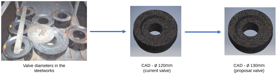
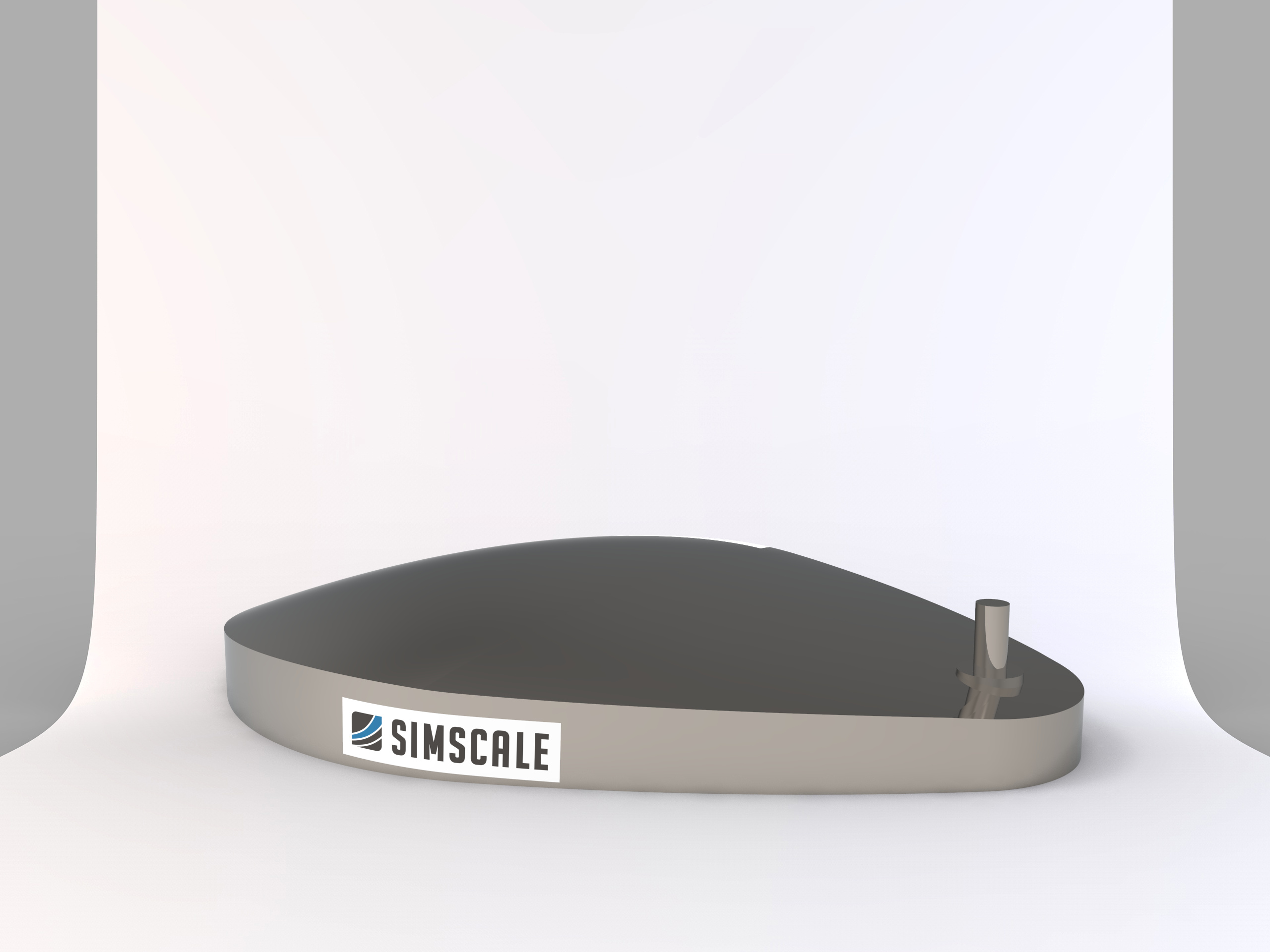
Figure 1: Valve geometry
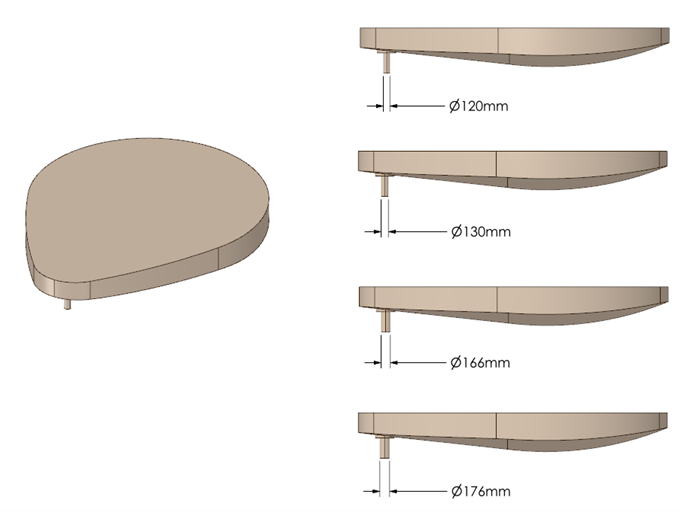
Figure 2: Fluid domains
\underline{\textbf{Meshing}}
Type: Hex-dominant automatic (only CFD)
\underline{\textbf{Simulation}}
Type: Multiphase Fluid Flow Analysis
The meshes of the models were executed with the Hex-dominant automatic algorithm used for internal flows, which minimizes the set of parameters of the original snappyHexMesh operation and sets the rest based on the CAD model, creating a polyhedral mesh quickly.
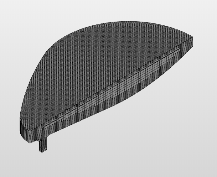
Figure 3: Hex-Mesh of the geometry
\underline{\textbf{Simulation Details}}
\underline{\textbf{Materials}}
\underline{\textbf{Boundary Conditions}}
The initial condition (time = 0 s) is exposed by Figure 4, with the EAF with about 40 tons of liquid steel, the condition of stopping the arrival in the liquid foot. In the case of an analysis of an incompressible, transient and non-heat transferable fluid:
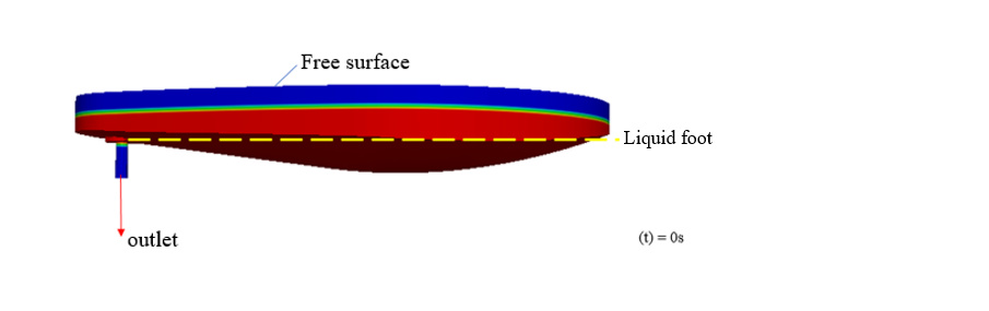
Figure 4: Boundary Condititions
According to the assumptions previously put, one can write the velocity by the equation of flow continuity, given by Navier-Stokes as:
In this case, because it is an incompressible fluid, the variable with respect to liquid steel remains constant with respect to time with a value, according to Widlund et al. (2011) of 6900 [kg / m³].
\underline{\textbf{Solution}}
Machine cores: 32
\underline{\textbf{Numerics}}
Numerical settings can be found inside the project!
\underline{\textbf{Results & Conclusion}}
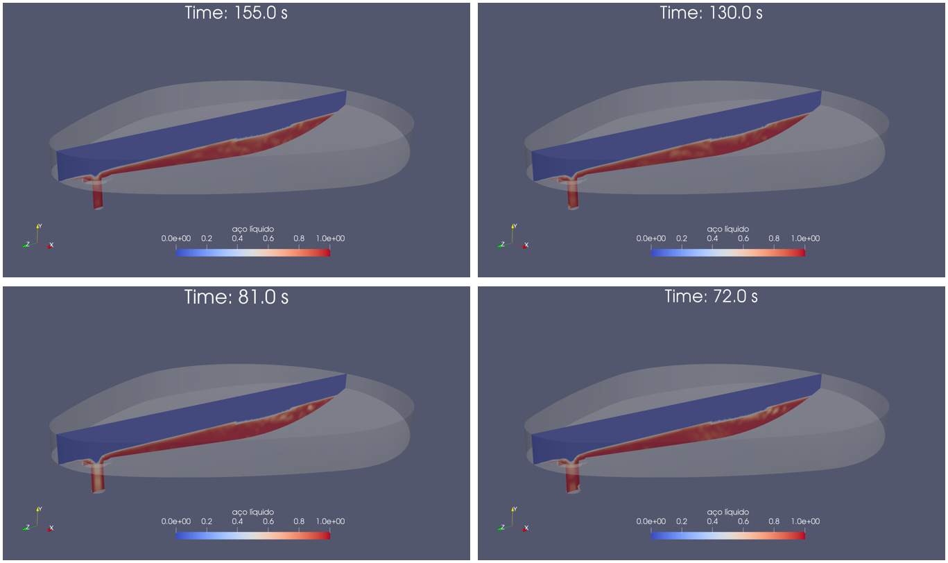
Figure 5: Run-off time up to the arrival in the liquid foot of steel for each valve
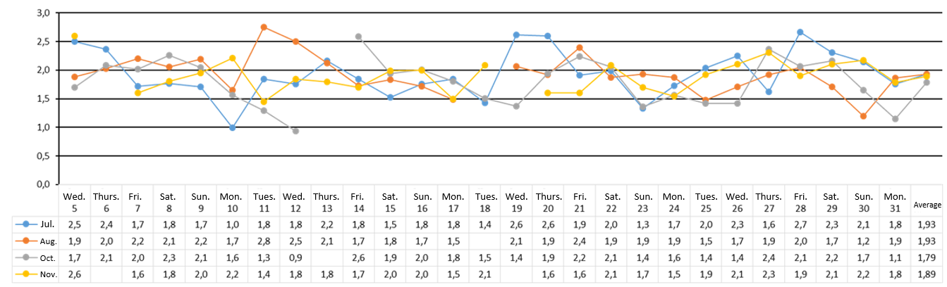
Figure 6: Flow rate for 4 months according to the different kind of valve
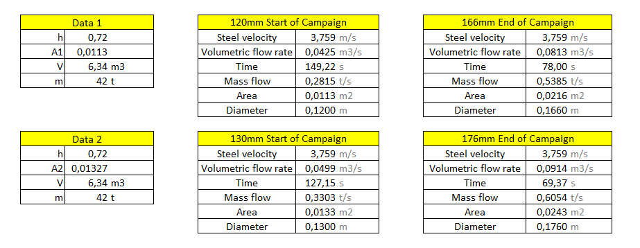
Figure 7: Experimental data to compare and validate the model
The experimental data was obtained through the furnace monitoring in the steelworks with the aid of measuring equipment (dimensions regarding the furnace and time), the flow being calculated through the equation of continuity given above. The months of July (blue) and August (orange) refer to the glove of 120mm, the month of September was discarded because it is a transition month and the months of October (gray) and November (yellow) refer to the glove of 130mm.
Figure 8: Results between different kind of valve
There was a reduction of approximately 25s with the 130mm glove, at the beginning of the campaign. At the end of the campaign, this reduction is minimized to about 10s. However, such results had a small variation, this is due to the repair done weekly in the glove, such repair aims to increase the useful life of the same and remained with a size of 120mm, which influenced the results collected in the area directly.
The validation of the CFD model via SimScale was compared with the results measured in the steelworks (Figures 6 and 7). It is verified that there is a small variation in the time of arrival in the liquid foot collected in the area in relation to the CFD. This difference is due to geometric approximations made to facilitate the discretization of the model, however, the value fluctuates in about 5 seconds translates a good convergence in the results.
\underline{\textbf{Sources}}
-
N. TIMOSHENKO, A. SEMKO & S. TIMOSHENKO. Modelling of electric arc furnace off-gas remote system. Ironmaking & Steelmaking. 2014; 41:257-261. Available in: http://dx.doi.org/10.1179/1743281213Y.0000000163.
-
O. WIDLUND, U. SAND, O. HJORTSTAM, X. ZHANG. Modeling of electric arc furnaces (EAF) with electromagnetic stirring. International Conference Simulation and Modelling of Metallurgical Processes in Steelmaking, 4, METEC, METEC InSteelCon, 2011. Available in: [PDF] Modeling of Electric Arc Furnaces ( EAF ) with electromagnetic stirring | Semantic Scholar
-
A. S. B. FERREIRA, V. S. GONÇALVES M. C. CARVALHO, G. C. RUSKY. Computational Simulation of the Lower Metal Housing of the Electric Arc Furnace of Steelmaking Sinobras S.A. ABM Week, 2º edição, 2017. Available in: ABM Proceedings - SIMULAÇÃO COMPUTACIONAL DA CARCAÇA METÁLICA INFERIOR DO FORNO ELÉTRICO A ARCO DA SIDERÚRGICA SINOBRAS S.A
\underline{\textbf{SimScale Project}}
To look at the simulation setup, please have a look at the project from @vgon_alves :
Multiphase flow in Electric Arc Furnace
To copy this project into your workspace, simply follow the instruction given in the picture below.

\underline{\textbf{Visit our SimWiki by clicking on the picture}}