Lateral Stability of Turbine Crop Duster (Thrush S2R)
Crop dusters are pretty amazing aircraft. Day after day, these airplanes are subjected to long hours, extremely high loading, and aggressive flight maneuvers. They’re also a segment of aircraft that hasn’t seen much in the way of the technological innovation enjoyed by GA and airliners. For the most part, the basic design of the two top manufacturers - Thrush and Air Tractor - has stayed unchanged for many years save for one: the conversion from radial piston to turbine engine power.
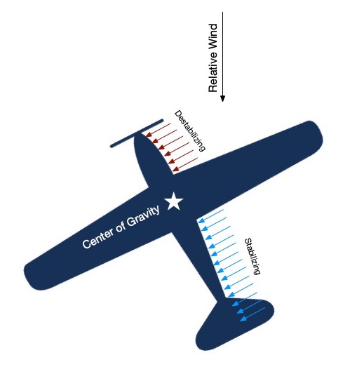
To convert an airframe from radial to turbine power is a non-trivial task. Radial powerplants usually have a power-to-weight ratio of around 0.5 hp/lb, where turboshaft engines are more in the range of 2 hp/lb. So for an airframe originally designed around a radial engine, the turbine must be locate further away from the center of gravity of the aircraft in order to maintain balance. The result is an overall lighter aircraft with more power and a pronounced extended nose. The extended nose is aerodynamically destabilizing because in a turn, it tends to be pushed around the turn by the relative wind. Here’s a cute little diagram:
For this project I wanted to analyze one of the most popular crop dusters, the Thrush S2R-510G. This is an enormous aircraft with a 500 gallon hopper capacity and the GE H80 engine with 800 HP. For those folks that know airplanes, I think you’ll find it significant that the empty weight of this aircraft is around 4500lb, while the max gross weight is 10500. That’s a useful load of 6000lb in a single seat aircraft!
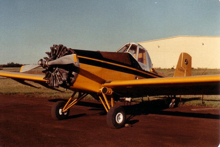
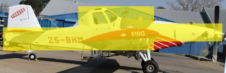
Here’s a photo of that airframe when it was powered by the venerable Pratt & Whitney R-1340 radial engine:
And here’s an overlay of that plane against the modern, turbine powered airframe:
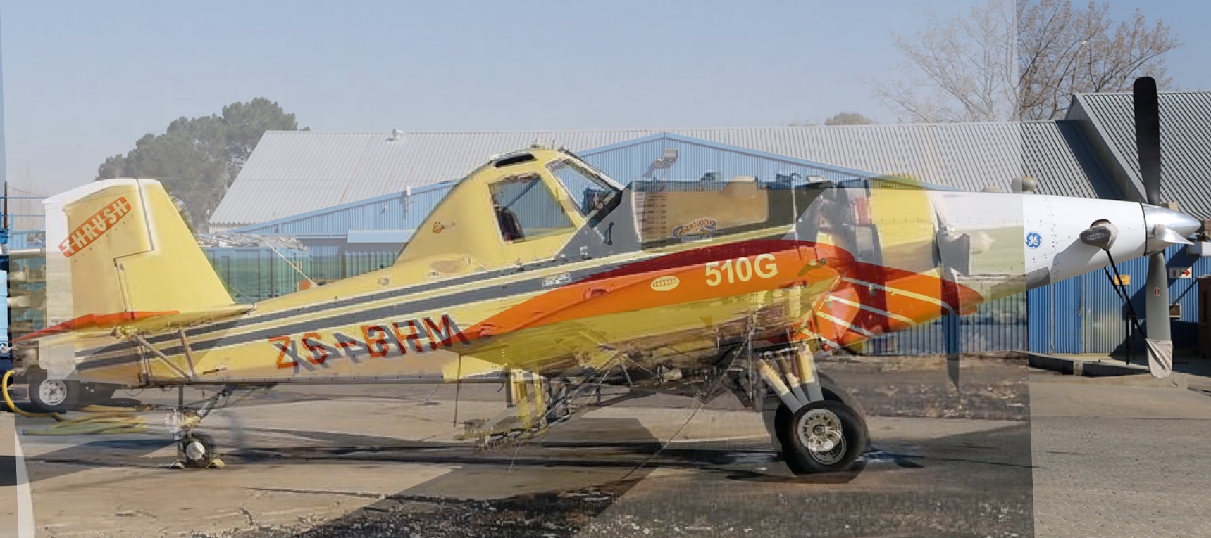
Note the massively extended engine cowling, much larger prop, and slightly enlarged tail volume to compensate.
So lets get to it!
I started with the Type Certificate Data Sheet to understand a bit more about this airplane.
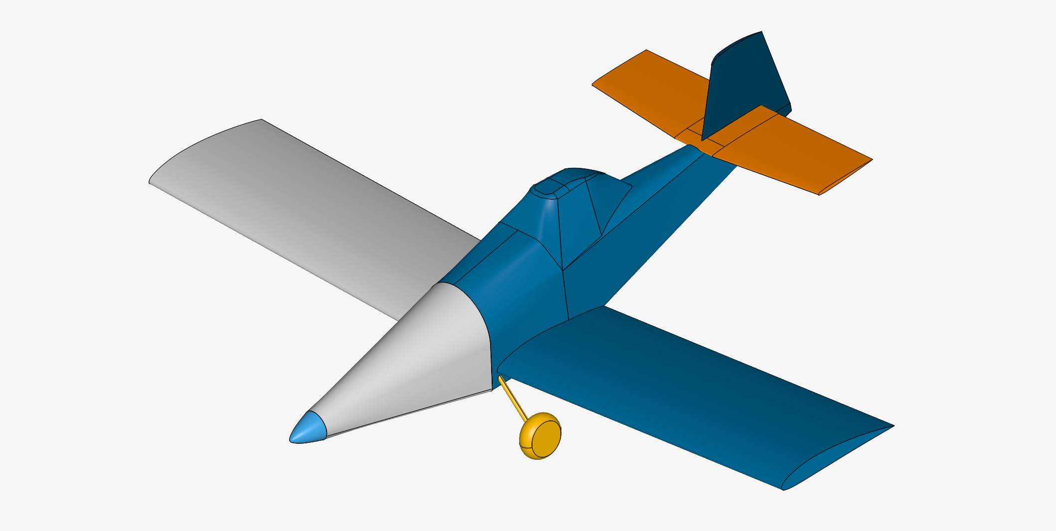
Then I made a model in Solidworks of the airplane by tracing the views I found in the maintenance manual.
Lesson learned: I originally followed SimScale’s docs on cad peparation but later went back and simplified my model even more. As it turns out, EVERY face transition has the effect of disrupting generation of the boundary layer when you go to mesh, so the fewer faces the better. For Solidworks users, this means a lot of fit splines and not worrying too much about fully defining sketches. Because of this, I do not recommend you try to use your primary mechanical model for CFD… you will just never get it decontented enough. Do yourself a favor and start out with a very, very simple geometric model. Take out EVERY feature you can, especially fillets and chamfers.
Lesson learned: There’s been a lot of discussion in the forums about CAD filetype export. I went with STEP file format, which seems to be about the same as IGES in terms of import. I did not try it, but I saw at least one user experience improved mesh generation when importing STL, which is a bunch of triangles already.
Here’s a shot of my model. Note the (mostly) seamless geometry. This model is still 74 faces and if I did it over I would find a way to simplify it further.
Setup
I wanted to understand the flow around the aircraft with a high angle of attack AND yaw angle that would be present when the aircraft is flying slow and making one of the banked turns at the end of a spray run. Specifically, I was interested in yawing moment, which helped limit my domain because I didn’t care about any of the other values such as pitching or rolling moment, or pressure forces.
Lesson learned: I recommend you get really honest with yourself here and be a real engineer. Like any engineering model, you’re unlikely to get something with perfect fidelity that magically eliminates the need for hand-calcs or scaled testing. On the contrary, if you try to solve all problems with this model you’re unlikely to solve any of them very well. Ask yourself how you an simplify the model at every step - can you exploit symmetry? Do you really need to model flow separation? Can the geometry be simpler? Can you analyze a subset of the geometry? Can you get useful results from a 2D simulation?
Meshing
I’m not going to lie: meshing was by far the hardest part of this project and the steepest learning curve. In this section I’m going to try to summarize the learning that happened as a joint effort in this very long, very detailed thread. I’ll present it as if I actually took a direct path there, but rest assured this was almost a month of work.
First, I learned a lot about Y+ and how it affects the validity of simulation results (hint: it’s a lot). This post from @jousefm is excellent, and you can find a bunch of resources from @LWhitson2 on this post.
A quote from @LWhitson2:
The Y+ calculation is a non-dimensional value that indicates whether viscous or Reynolds stress is more important to the flow.
* Viscous Dominated: 0 < Y+ < 1 (Full Resolution)
* Mixed Stresses: 1 < Y+ < 50 (Avoid this region)
* Reynolds Dominated: 50 < Y+ < 200 (Wall Functions)When the boundary layer calculations are based on the mesh size, the first layer thickness will change. It is very easy for the layers to fall into the Mixed Stresses region without the user knowledge. In the end, the goal is to fall within either the Full Resolution or Wall Functions layer with your first point from the wall.
Lesson learned: Correct boundary layer modeling is what makes the difference between pretty pictures and useful results. Embedded in the solvers are assumptions around the characteristics of the boundary layer. These assumptions can be extremely wrong in some cases, so it’s important to actually understand the Law of the Wall and Y+ thoroughly.
I did some initial rough tests that were enough to give me confidence that flow separation was important to model. The fuselage was causing a large turbulent area that affected even the horizontal stabilizer. Unfortunately, this meant that I needed to do a full resolution analysis with Y+<1 for my first layer.
Away to the calculator! I used this online calculator. BE SURE TO FILL IN THE DEFAULT VALUES FOR AIR FROM SIMSCALE. Be aware that SimScale uses Kinematic Viscosity but the calculator uses Dynamic Viscosity, which are related by the following equation (thanks @DaleKramer) :
Kinematic Viscosity * Density = Dynamic Viscosity
The density and kinematic viscosity values are slightly different, so this can cause differences from your model. Here’s an example of my results for Y+=1. That’s a first layer thickness of about 0.01mm, so very thin.

Next I followed @DaleKramer’s method of mesh generation, which I affectionately refer to as the Kramer Method. Read that post before you attempt mesh generation and then follow it exactly.
Here’s the problem: SnappyHexMesh is the mesh generator used by OpenFoam/SimScale and it loves to throw away cells. Basically it takes your raw geometry and overlays a bunch of hexahedrons. Then it assesses how much of the hex cells are impinging on geometry and either splits them up or deletes them altogether. It does this iteratively until it hits an iteration limit or it achieves your mesh quality criteria. Then it blows up a beautiful and complete set of boundary layer cells out of the surface cells and starts to follow the same process. Unfortunately this means you watch as it kills off most of your precious BL cells and you cry into your coffee cup. At least that’s how it went for me.
Here’s what worked:
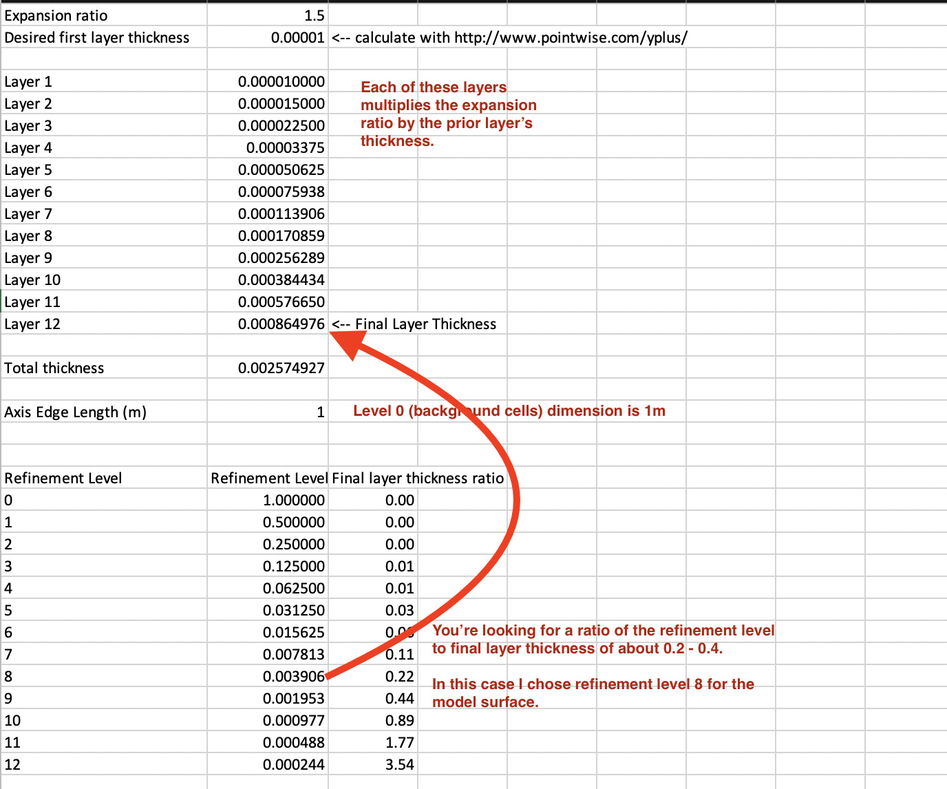
- Determine my background mesh box cell dimensions. THESE SHOULD ALWAYS BE CUBES. In my case, I found that 1x1x1m cells gave me a good balance between detail of the model and overall cell quantities to fit within my 32 core limit.
- I made a spreadsheet of refinement levels, first layer thickness, and expansion ratio. SimScale uses the concept of refinement levels for mesh refinements, so basically it takes the background mesh box cell dimension and starts dividing it. Here it is for 1m cubes:
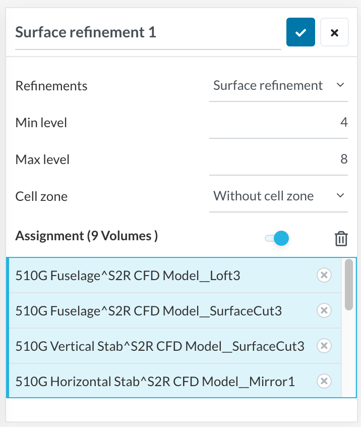
- Set up my mesh in Simscale with only the following refinements:
Surface refinement
In this case, I used a variable surface refinement. This does limit BL generation a bit as it’s more transitions between large and small cells, but I considered it worth it as it reduced my number of cells by around 50%. If I was doing a small model or thicker BLs, I would have done a uniform refinement of 8-8 instead of 4-8.
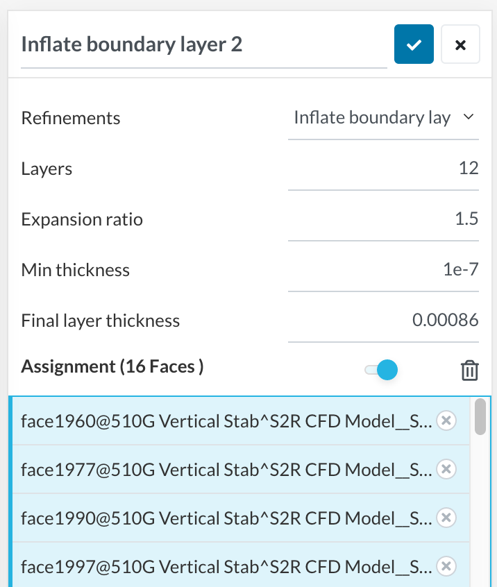
Boundary Layer Refinement
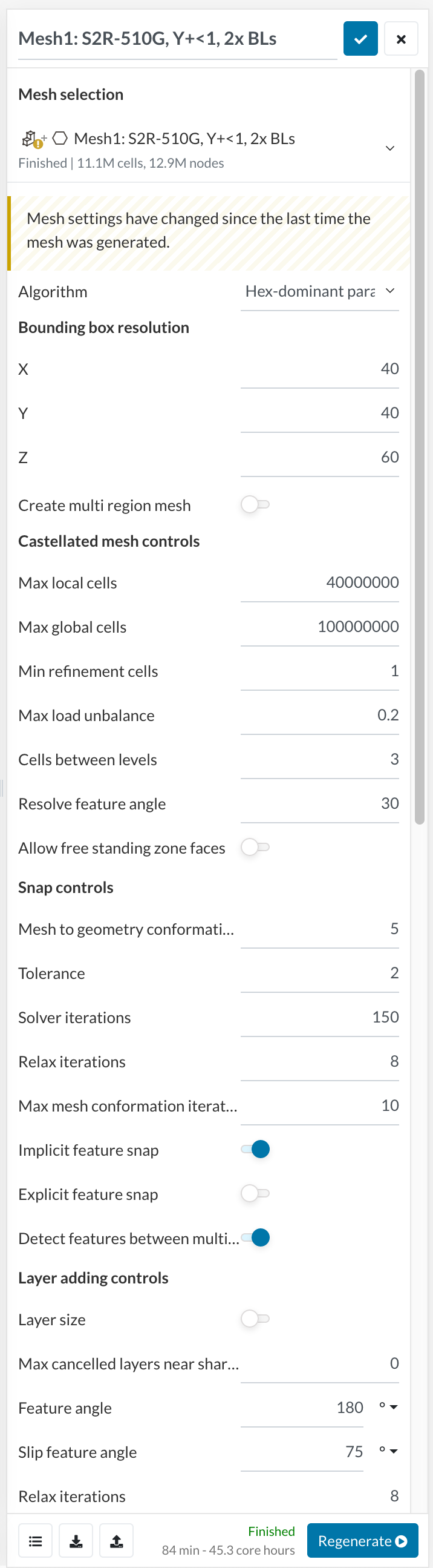
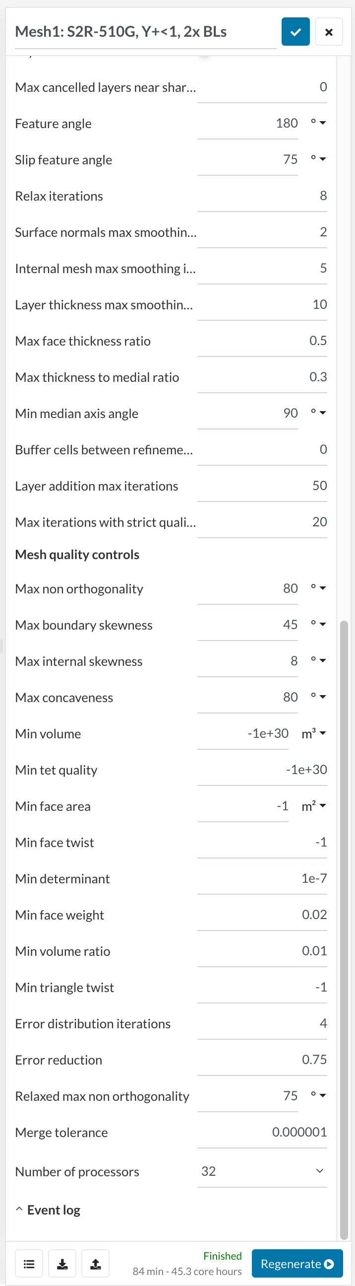
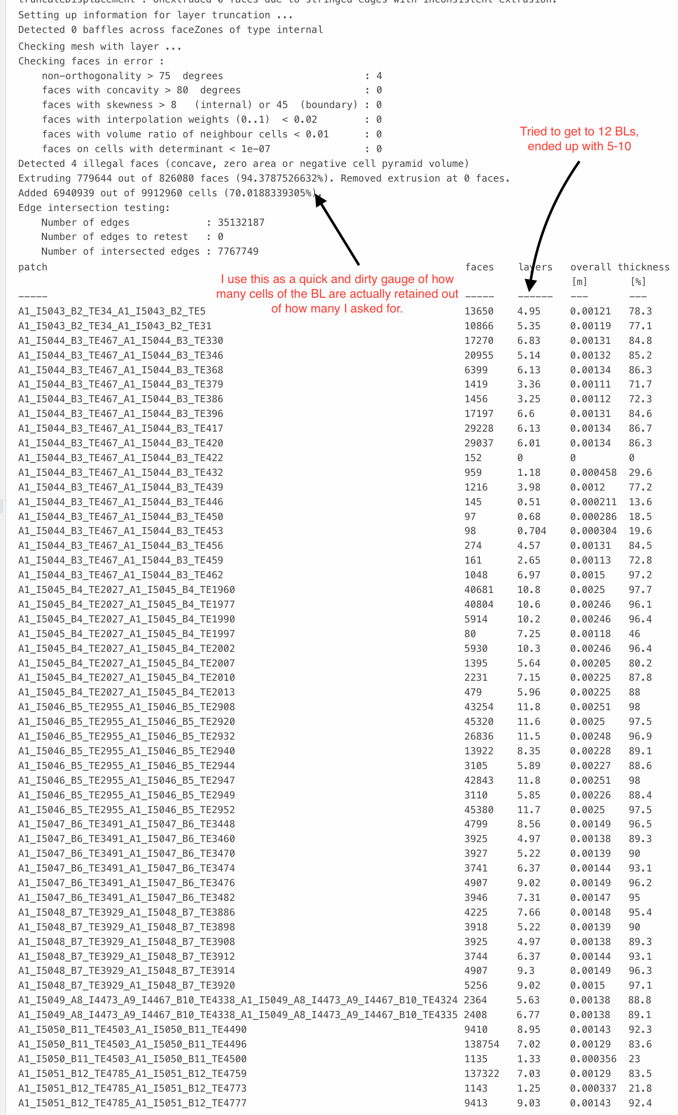
This should mostly match what I developed in the spreadsheet. - Time to generate the mesh! This is an iterative process in which you watch the meshing log and then loosen mesh quality checks while trying to avoid mesh errors. In the meshing log, you will usually see a line where it shows a bunch of cells away due to mesh quality checks. These might be for face twist, volume, max determinant, etc. Once you see that, you can loosen the quality check and you will It can be time consuming and frustrating, but in the end you will get a good BL. Here’s the settings I used for this mesh, which came out to around 70% coverage.
Here’s a shot of the meshing log:
So you can see here that coverage wasn’t great but it was pretty good compared to my original attempts. Because I still didn’t have super high confidence due to the low retained cells, I decided to do a bit of a mesh invariance study. Basically I tried a couple different mesh refinements, including using wall functions (Y+=120). Generating meshes on those were WAY easier with more retained cells. The thinner the BL the more cells that Snappy throws away.
Simulation
Okay now for the simulation part (finally!). I chose K-omega SST and set initial conditions for K and omega that I found in a few other simulations. At some point I checked them but I have forgotten where that resource was.
For the model, I set a no-slip wall condition.
Lesson learned: you can right click in the model area and hide faces or features. It’s often faster to hide a couple features and select all visible… just be sure for your BL generation that you aren’t selecting faces that are coincident with other faces or hidden.
Crossflow
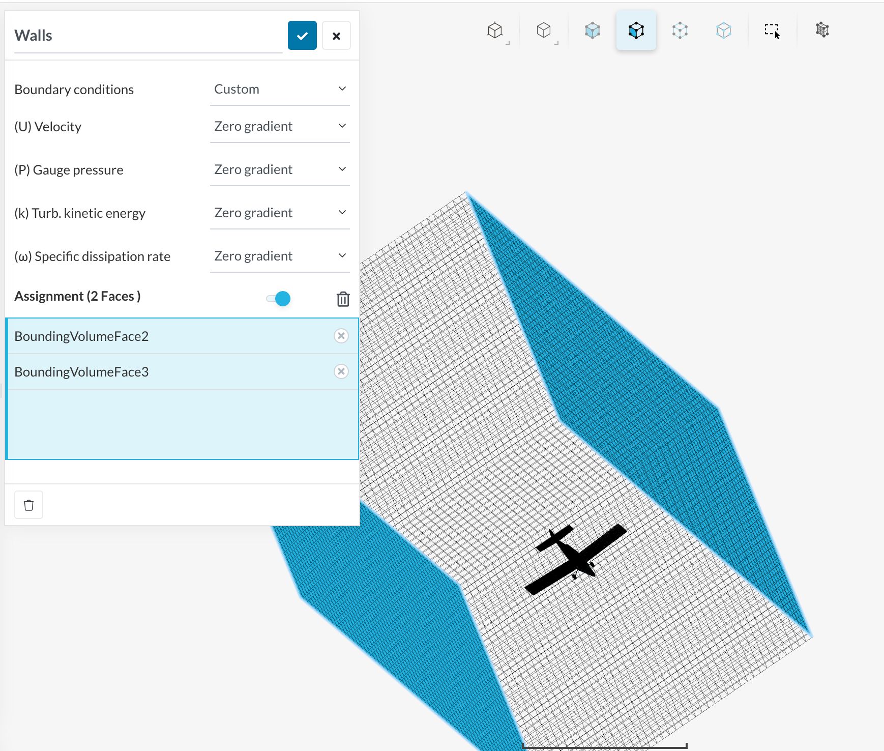
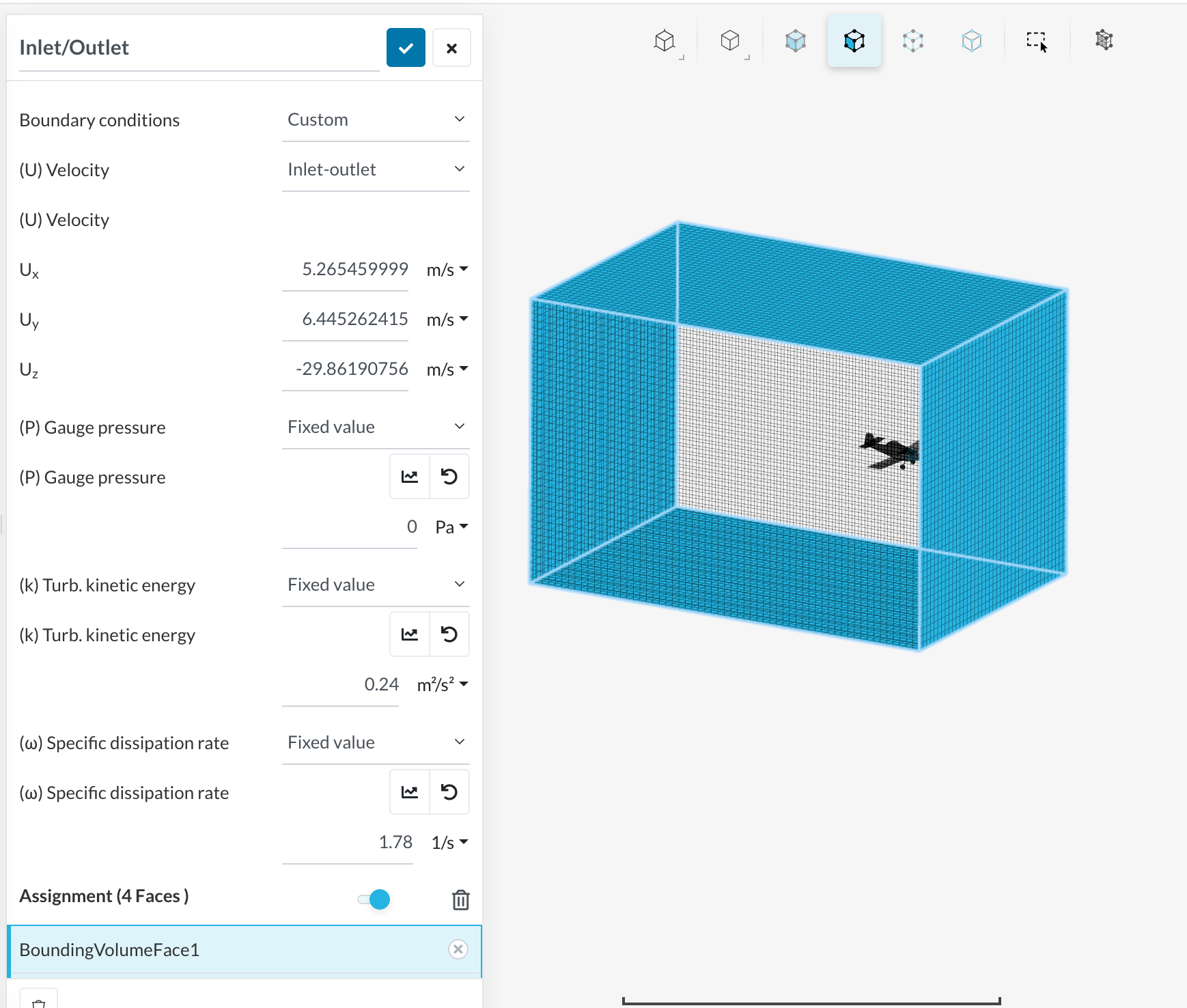
Because I needed a crossflow condition and there is no way to re-orient the model, I had to set up the walls to flow with a special condition. If you’re not doing straight-on flow, you’ll benefit from this approach which I think was suggested by @LWhitson2. I set the side walls to zero gradient and the front, bottom, back, and top walls to a custom inlet/outlet condition calculated flow vector which I got through… trigonometry! This allowed the flow to move unimpeded across my background mesh boundaries and seemed to help convergence over using other methods I gathered from SimScale examples. So if you have a flow that is NOT solely in one direction, consider this method.
Results
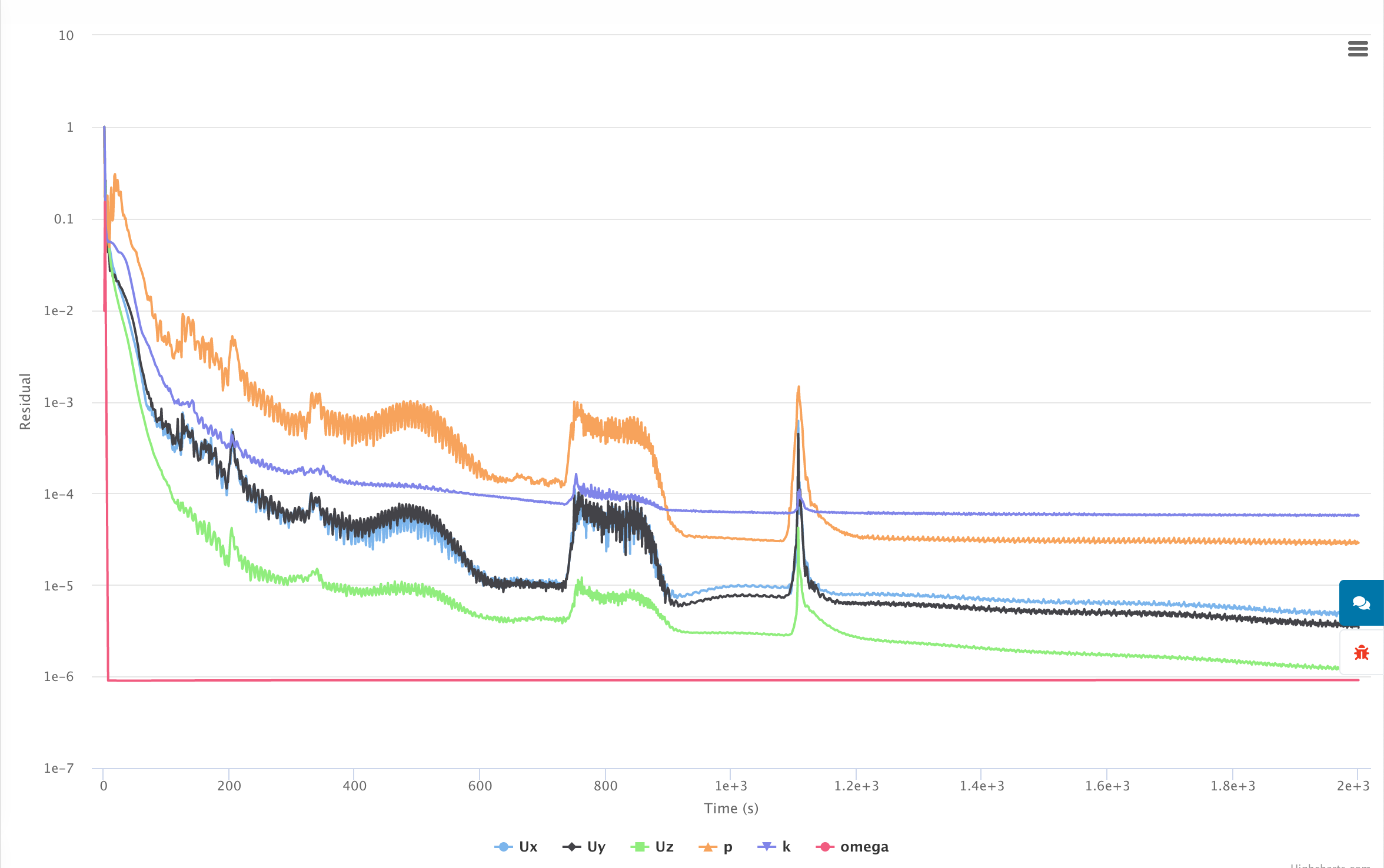
I experimented a lot with run times and found that I needed an unreasonably long time to reach stable values for this model… well after the model had converged. For the Y+<1 run we’ve been discussing, I ran 2000 timesteps and still saw values climbing slightly but they were stable enough for my purposes. Here’s the plots:
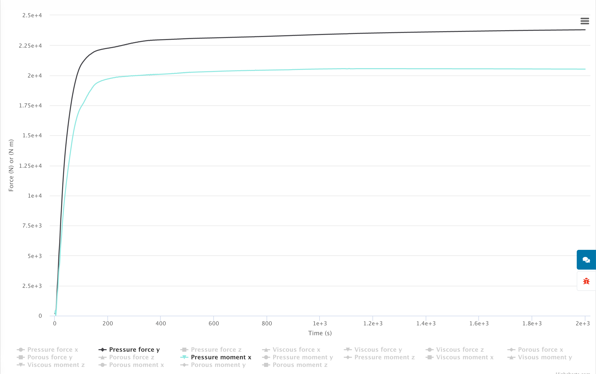
We’re getting around 24000N of lift, or around 5400lb which is about 1000lb over the empty weight of the aircraft. That’s a good sign!
Convergence happened relatively early. I probably could have run longer.
Lesson learned: Early on in running these simulations I had issues getting them to converge. Then someone recommended I try turning off Simulation Control>Potential Foam Initialization. This worked fabulously well.
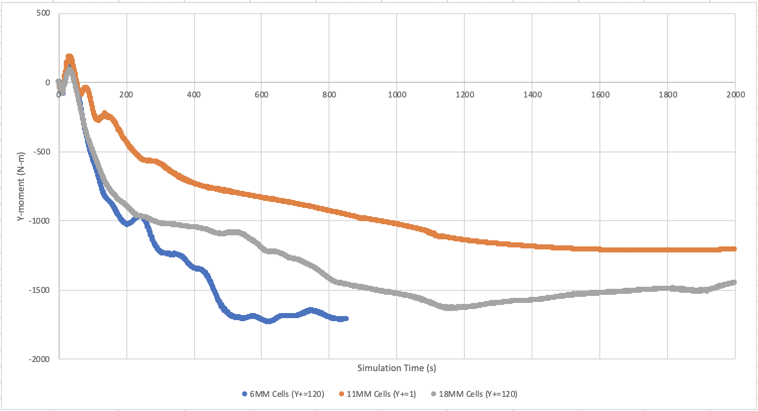
Here’s the plot of y-moment (yaw) between the three meshes. You can see that the coarsest mesh comes in at around 1700Nm where the y+=1 mesh comes in at around 1250Nm, or about a 25% spread between them. I’m not sure if that’s normal, but in all the simulations I did (and there were many, many more than this), this spread and the absolute values were very similar between the low resolution and high resolution BLs.
I would really like to show some images of Y+ and the flow separation, but for some reason SimScale’s post processor is not working at all. I’ll add these when it starts working again. For now you’ll have to go into the project itself and take a look.
What you’ll notice from the flow patterns in all the simulations is that the vertical stabilizer shows very little pressure differential, indicating it’s probably not especially effective due to blanking from the fuselage. Similarly, there is a massive separation zone at the wing-fuselage intersection on the leeward size which appears to blank the horizontal stabilizer. Since I didn’t investigate pitching moment, there isn’t a way to tell the effect of this, but I would expect the tail surfaces to be only marginally useful at these AOAs.
Corroboration
I’m always skeptical of simulation results and feel strongly that they should always be corroborated with hand calcs and testing. It’s common practice now for young engineers to forget the valuable work they did in hand-calcs for the convenience of computer simulations. Garbage-in, garbage-out as they say.
I attempted two methods of hand calculations in order to give myself some context and confidence. My approach was to divide the fuselage into a set of simple rectangular shapes like below:
Because the vertical stabilizer has such a large effect, I decided to neglect it until after I had results I liked for the fuselage.
My first analysis was with the fuselage as a set of flat plates with angle of attack matching the beta angle of my CFD simulations (12º), using the standard 2*pi*beta drag correlation. The result for the fuselage with this correlation was 2234 N-m (1648 ft-lb). I’d expect this approach to estimate high, as the fuselage is better modeled as a slim lifting body.
The next analysis was using an old paper, NACA TN4176. In this paper, they develop a method to use drag correlations taken from cylinders with a variety of cross-sections to estimate drag on similarly shaped fuselages at different pitch and yaw angles.
For this analysis, I used the correlations for three rounded rectangular cross sections with the same aspect ratios as the flat plate analysis. This approach yielded a yawing moment of 871N-m (643 ft-lb), bracketing the other side of the CFD results.
Again, neither approach took into account the contribution of the vertical stabilizer, which is probably the biggest contributor to lateral stability. Adding the stabilizer in as a flat plate dramatically skews results toward stability (as it should), but from the CFD flow pattern I observed, I’m not convinced it’s especially effective. I think the vertical and horizontal stabilizers are receiving separated flow from the fuselage and cockpit, so their effectiveness would be reduced.
Discussion
I hadn’t done any complex flow simulation beyond tutorials and simple Solidworks 2D stuff prior to this project. After about 30 days of continuous iteration and a TON of help from the PowerUsers here on the forum, I arrived at results that are acceptable, though far from definitive.
It’s dramatic how much effect the proper configuration and generation of the boundary layer had on the results. It’s also dramatic how difficult it is to get this platform to generate a quality one. After all the work on it, I think it really comes down to clean geometry. If you follow @DaleKramer’s excellent work on this, you’ll notice that his geometry is nearly seamless whereas mine has many, many faces.
For new users, I’d encourage you not to look upon CFD as a quick solution to hard problems. It’s exceptionally easy and fast to make a pretty picture, but extremely difficult make one that corresponds well to the real world. If you’re brave enough to continue on, I hope my experience on this project will prove useful.