Correlation issues

[akosior]

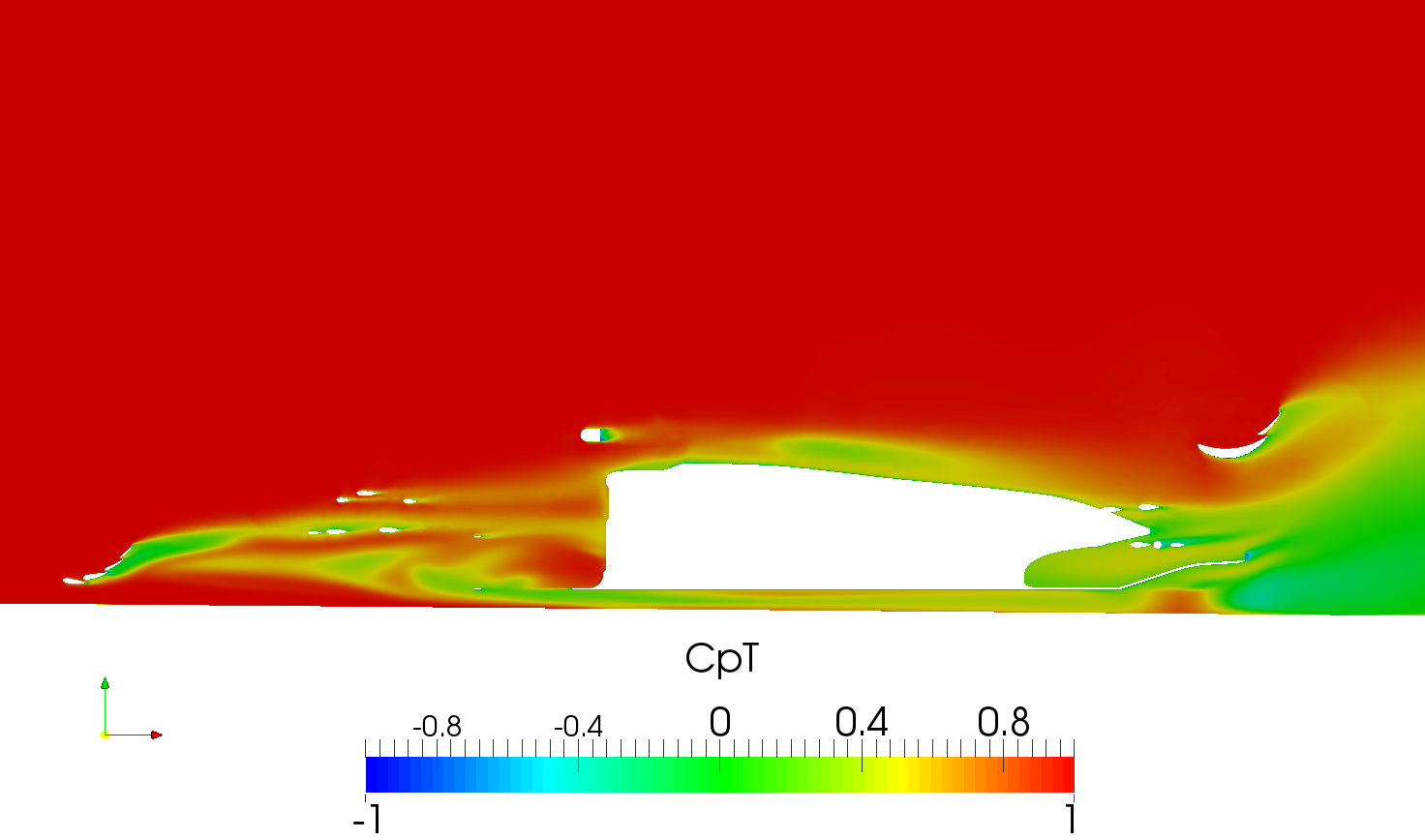
As we have done some simulations and got results for our F1 car we run into correlation issues. There are two main differences in comparison to other CFD software:

• flow separation point on the top of the tire is much later,
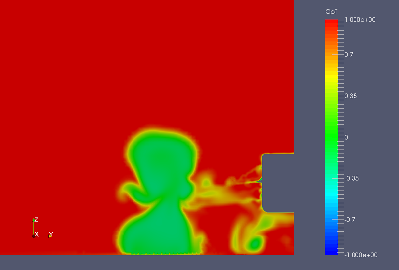
• there is no stall region behind the rear wing.

We think that there may be two reasons for that. First one is the coarse mesh (11M in comparison to 20/50M for the ohter software). I know that the fix for the creation of the fine meshes is just around the corner (Recover Successful Mesh Computation but Error After - #5 by dheiny). The second problem might be using the first order upwind scheme. The solution would be to use higer order schemes but the computations does not converge when using linearUpwind or vanLeer. Normally we could start the computations with the first order scheme and after some time restart them with a second order scheme. Unfortunatelly this feature is still under development (Restarting simulation if convergence isn't reached - #4 by dheiny - @dheiny: Do you have any news on the release date?).

Does any of you have some suggestions on what else could be the source of those correlation issues or how can we fix them?

[AnnaFless]

@Ali_Arafat or @gholami any ideas here?

[dylan]

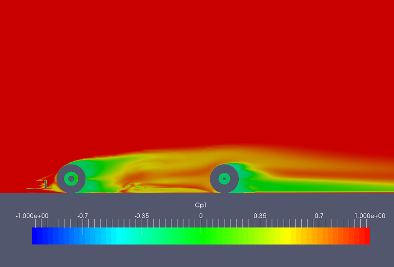
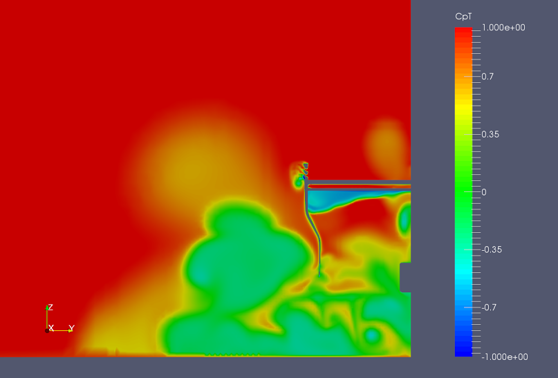
1) flow separation point on the top of the tire is much later

• It is hard to tell where flow separates along the tyre centre-plane with a total pressure coefficient contour, specially on a rainbow colouring.
  a) Rainbow is confusing with its green part.
  b) You need to plot Cp vs Theta on the tread to find the saddle point according to Fackrell and Harvey (1974).
  c) What flow separation angle did you expect - between 285 and 290 degrees reading anti-clockwise with zero degree at the most upstream location?
  d) On the tyre centre-plane, use Cp between -1 and 3 normalised by free stream dynamic pressure. The coefficient is above unity in this incompressible flow. It is not common to have Cp > 1 in incompressible flow unless there is work done on the system. In this case the moving ground plane does work on the tyre near its contact patch.
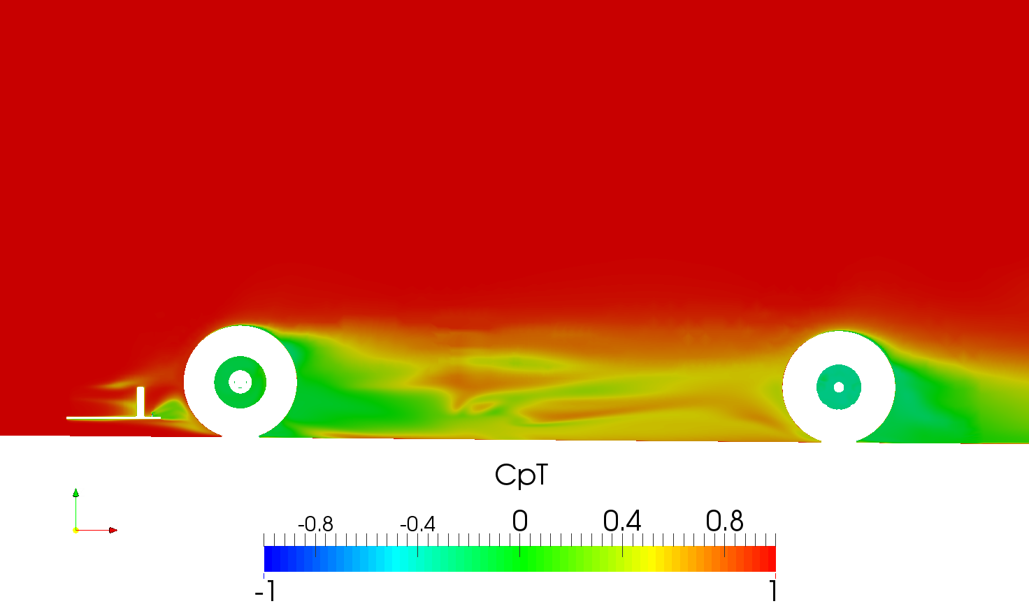
  e) You would expect a highest Cp value at least 2.0 depending on how ‘tall’ your contact patch step is.
  f) You need a lot of cells around the contact patch to capture this high pressure in order to capture the jetting phenomenon, which also affects the downwash of the flow coming off the top of tyre tread and reflects the tread separation location.

Here, read this paper: Sammy Diasinos, Tracie J. Barber, Graham Doig, The effects of simplifications on isolated wheel aerodynamics, Journal of Wind Engineering and Industrial Aerodynamics, Volume 146, November 2015, Pages 90-101

2) there is no stall region behind the rear wing.

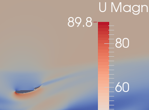
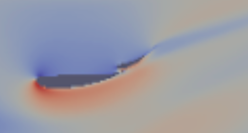
• You front wing looks the same - same kind of wake - and how do you easily tell flow separation? Try to look at velocity contours instead of CpT contours and expect velocity distribution of a positive overhang flap. In all my solves, realizableKE was able to predict the rear wing.

Flow is mostly attached on the rear wing below:

3) The solution would be to use higher order schemes but the computations does not converge when using linearUpwind or vanLeer.

• It is not uncommon. Maybe switch off the limiter in the gradient of div(phi, U) when using 2nd order upwind. I can see that on your 25M mesh there are non-orthogonal cells above 70 degrees and you have used limited scheme on the viscous terms.I believe if a case is set up properly and will converge, then starting with 2nd order upwind will also converge. If it still fails, try limitedLinearV.

In terms of the gradient terms, maybe use leastSquares instead if you take away the limiter on the gradient of the convective term.

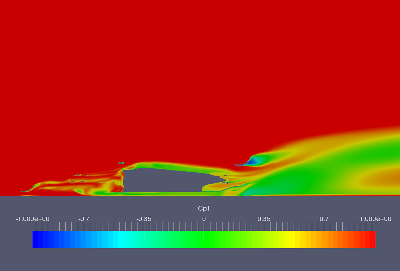
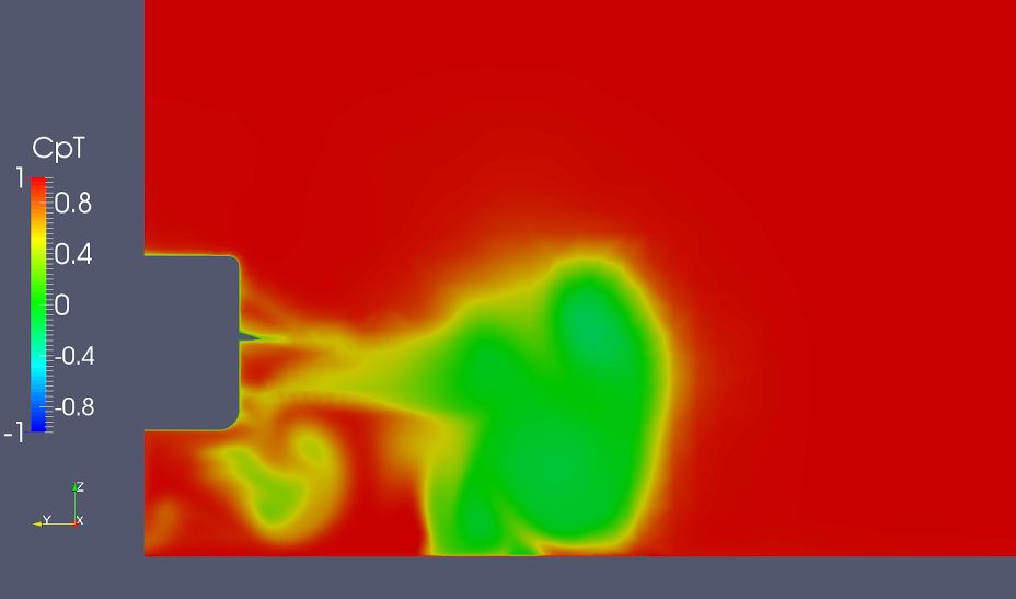
Added: my bad here. I didnt know which slice you were referring to. After looking at In-house OF32 with 33M and 5 layers, the ‘not stalled’ rear wing does look like a mesh resolution issue.

your post

I also found the slice for the tyre on In-house OF32 with 33M and 5 layers

your post

The In-house run has a much clearer main and tread vortices and a taller and more skinny front wheel wake, consistent with the wake features associated with a rotating wheel in contact with a moving ground.

[dylan]

I had a quick look at your results:

In-house OF32 with 33M and 5 layers: good main and tread vortices

simscale OF231 with 11.2 M: the outboard jetting seems weak. can’t really see a good pair of main vortices

So it does look like a resolution issue.

By the way, on In-house OF32 with 33M and 5 layers, I can see the unhappy-looking rear wing now:

[akosior]

Hi @dylan,

great post (two actually). I had some points but then you answered them yourself . As you can see for now it is rather verification than interpretation of the results that we are looking at. The results that you showed from your in-house cluster are what we are hoping for to get at SimScale. Can you share configurations of your run (turbulence model and schemes)?

Best,
Andrzej

[dylan]

Hey @akosior, the results from my end were not an F1 car but various closed wheel autocross racers. I had a look at your case setup on the 25M run, the major differences were we use: 1) SIMPLEC, 2) realizableKE, 3) 4~5 boundary layer cells on upper/underbody and front/rear wings, while 2~3 layers on wheels. We also have more choices on discretisation schemes but for all the steady state simulations, good results have been obtained with linearUpwindV, limitedLinearV, and gammaV.

25M or more on half an F1 car sounds about right (probably with only 2~3 layers on the whole car?), but the spreadsheet doesn’t have this entry? Did your mesh end up with 25M cells?
If not, it might have been an resolution issue.

[akosior]

Hi @dylan, I meant the configuration of the run from which figures you posted.

The 25M in the name was the maxGlobalCells setting but it got to about 11M. We had problems with finer meshes creation on SimScale (but the fix is on the way). This is why there are only 11M runs in the spreadsheet. There is a tab called ‘Spec’ in it, where the specification for the mesh is given (for now it is 2 layers for the body and tires, 5 for wings, ground and contact patch).

[dylan]

Hi @akosior, by configuration of the run do you mean fvSchemes? I don’t think the car geometry is of your interest, because it is not an F1 car.

fvSchemes on a good mesh:

ddtSchemes
{
    default         steadyState;
}

gradSchemes
{
    default         Gauss linear;
}

divSchemes
{
    default         none;
    div(phi,U)      bounded Gauss linearUpwindV grad(U);
    div(phi,k)      bounded Gauss upwind;
    div(phi,epsilon)  bounded Gauss upwind;
    div((nuEff*dev(T(grad(U))))) Gauss linear;
}

laplacianSchemes
{
    default         Gauss linear corrected;
}

interpolationSchemes
{
    default         linear;
}

snGradSchemes
{
    default         corrected;
}

fluxRequired
{
    default         no;
    p;
}

fvSchemes on a bad mesh:

ddtSchemes
{
    default         steadyState;
}

gradSchemes
{
    default    Gauss linear;
    grad(U)  cellLimited Gauss linear 1;

  // with gamma differencing
   default    Gauss linear or leastSquares;
}

divSchemes
{
    default         none;
    div(phi,U)      bounded Gauss linearUpwindV grad(U);
    div(phi,k)      bounded Gauss upwind;
    div(phi,epsilon)  bounded Gauss upwind;
    div((nuEff*dev(T(grad(U))))) Gauss linear;

 // with gamma differencing
    div(phi,U)      bounded Gauss gammaV 1;
    div(phi,k)      bounded Gauss vanleer;
    div(phi,epsilon)  bounded Gauss vanleer;

}

laplacianSchemes
{
default Gauss linear limited 0.5; 
}

interpolationSchemes
{
    default         linear;
}

snGradSchemes
{
    default         limited 0.5;
}

fluxRequired
{
    default         no;
    p;
}