Proper handling of multi-solid domains
Multi-solid domains have to be connected in order to run a mechanical or thermal analysis. How to set up those connections often causes troubles. Do I have to prepare the geometry in my CAD-system already? Can I connect multiple bodies in one conform mesh (with shared interfaces) and still keep them distinguishable in order to assign materials or boundary conditions? As poorly defined or missing connections often cause errors or strange results I want to explain the different mechanisms quickly with a hands-on example: A thermal analysis of a resistor assembly. Please feel free to ask questions and comment on all addressed topics. Especially your feedback and suggestions how to ease the workflow are highly appreciated!
The incentive for this forum post came from a constructive discussion with @kturnbull and his project resistorassyinbox by kturnbull | SimScale. Special thanks to him for providing his geometry and setup which fits very well for showcasing the topic. You can also have a look at my modified project here: resistorassyinbox by afischer | SimScale
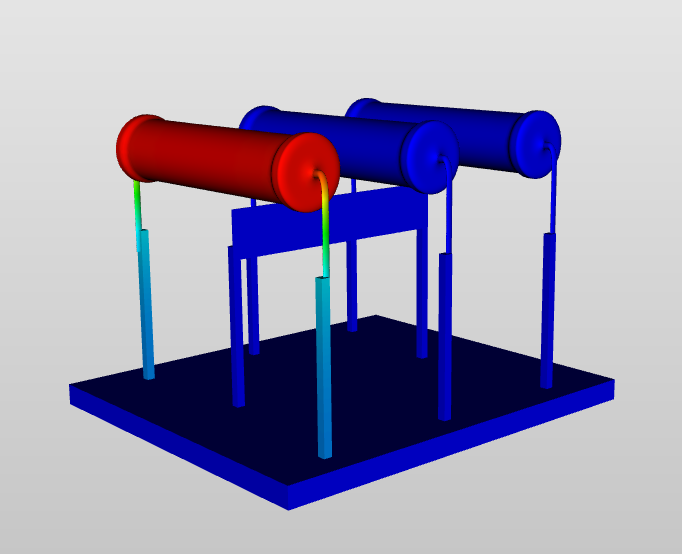
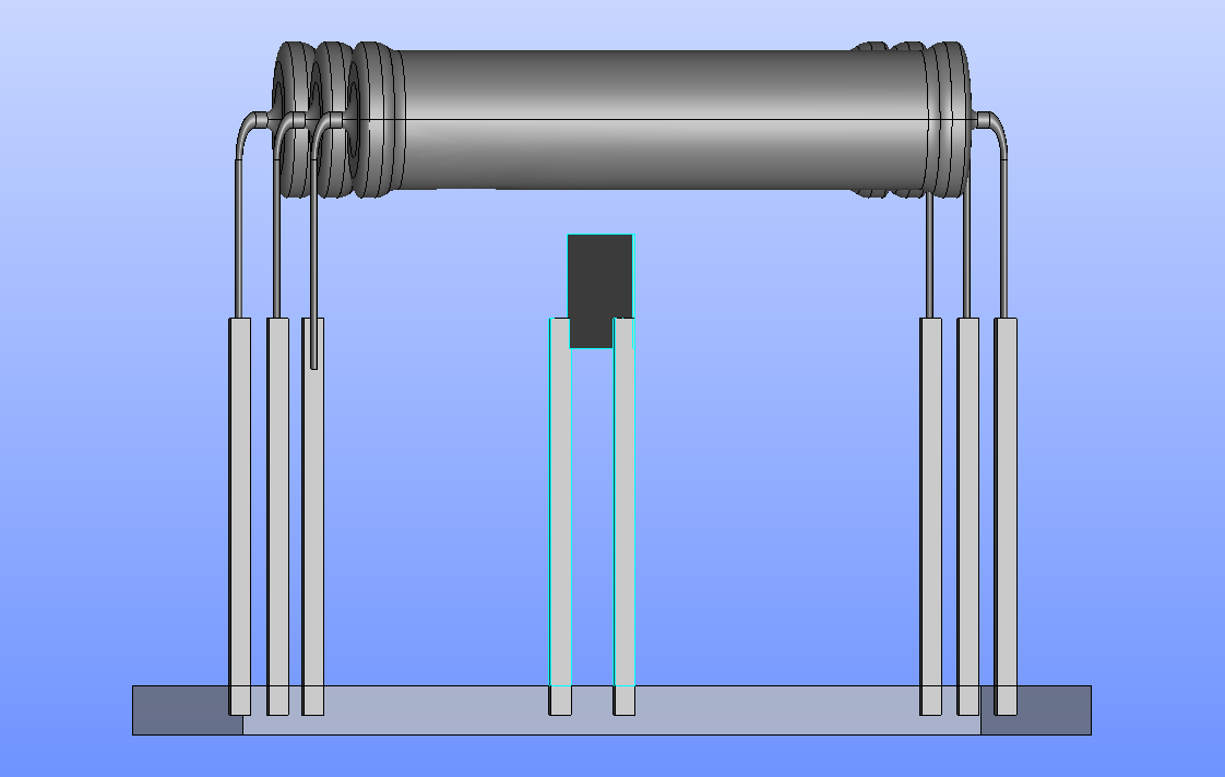
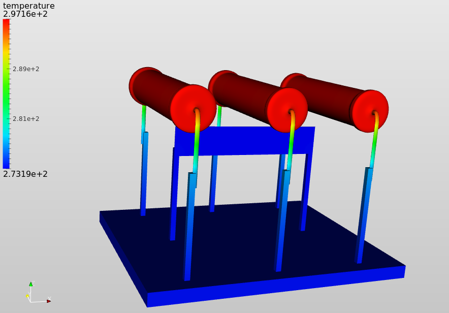
Temperature distribution in the assembly with proper boundary conditions but missing connectivity.
When running simulations on a solid body, the domain has to be first discretized. After the meshing the domain consists of a number of elements/cells that are connected inherently via shared faces, edges, nodes etc. . In case of a finite element analysis the solution field (e.g. the nodal displacements in a mechanical setup or temperature values in a heat transfer analysis) is computed afterwards for all nodes of the mesh.
In most cases the geometry does not consist of a single body but a so-called assembly of multiple bodies. This makes sense both from a modular design approach as well as simply the fact that those bodies might have very different properties e.g. materials. In the simulation setup you can easily assign those properties to the corresponding bodies. However you have to take care that the different mesh parts are either connected via shared nodes (a so-called conform mesh) or that contact constraints are added in the simulation setup in order to couple the solution at the interface numerically.
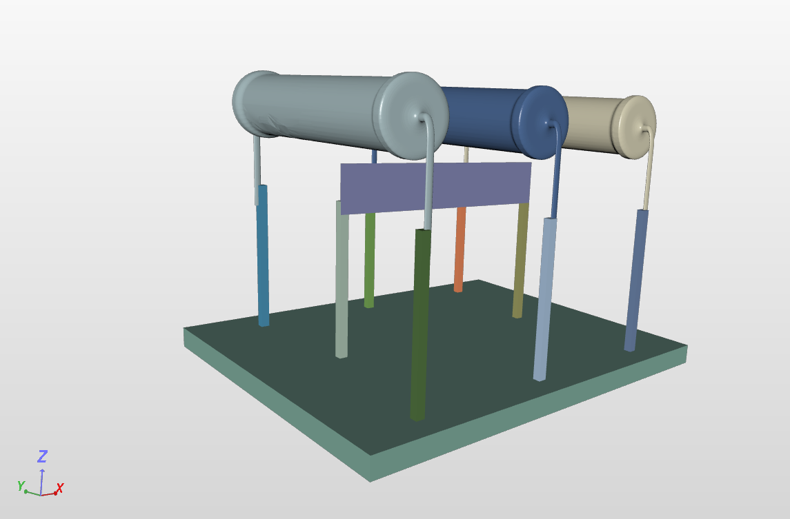
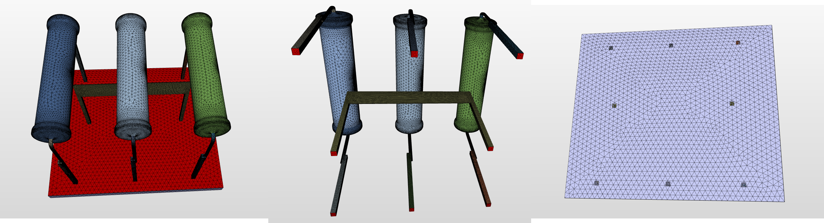
Assembly consisting of 12 solid bodies indicated by the coloring.
Generally there are three different ways of coupling parts together, two of them can be classified as CAD preparation, while contact constraints are a numerical way of establishing connections.
- Fuse bodies
A fuse operation combines multiple bodies to one body, reducing the problem simply to a single-body setup. It results in one mesh part that does not allow to differentiate between the original parts anymore. Although the interface entities (e.g. edges in the image below) are often preserved the mesh-clip shows that generally the interface between the original parts is not existent anymore. You should be able to perform fuse operations (a boolean operation) in almost every CAD-tool.
Fused bodies are meshed as one solid (see color indication)
- Multibody / Non-manifold / Partition
There are many different names for this connection type, so lets focus on the actual characteristics. A Multibody consists of multiple parts that share entities at their common interface. It results in a conform mesh (common nodes on the interface) where the original parts are still accessible, thus combining both advantages. It is a more complex geometrical operation though that might not be available in every CAD-tool and causes troubles for some CAD-formats when exporting.
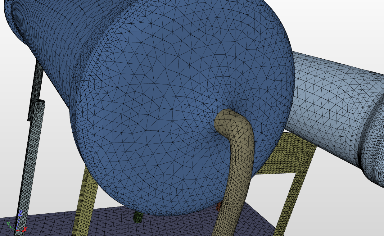
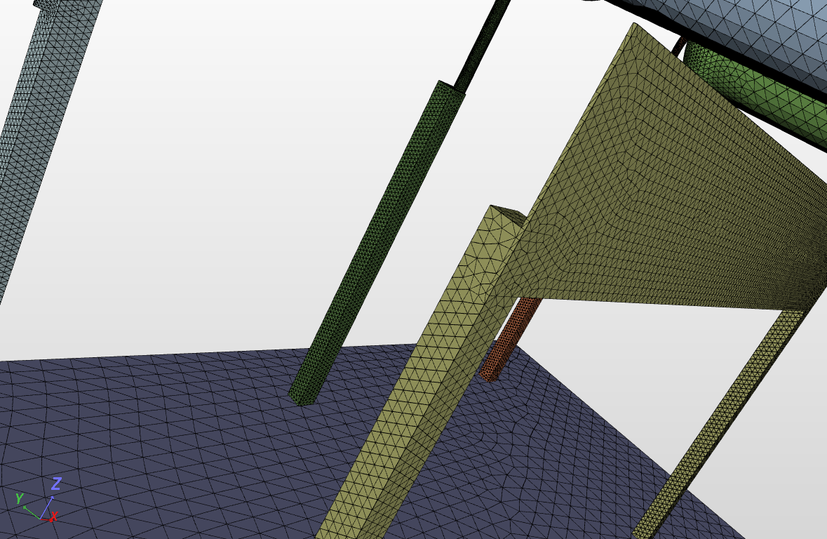
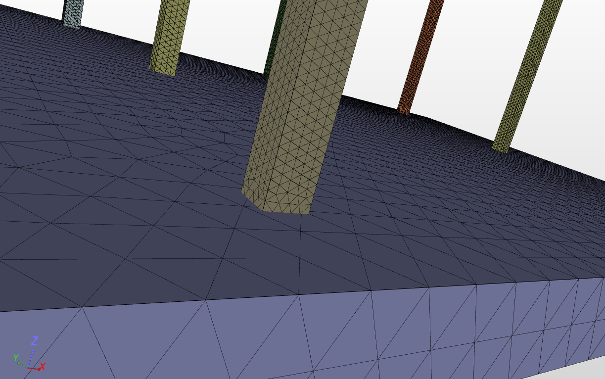
Two differentiable bodies (indicated by coloring) combined in one conform mesh. The parts share nodes and lower dimension elements (surface elements in this case) on the interface.
- Contact constraints
Contact constraints combine two mesh parts numerically by establishing multiple point constraints between the nodes of both parts in the interface region. That means there is no connection in the mesh itself. It is applied in the simulation setup and is therefore only valid for the corresponding simulation. You can easily copy those for a new simulation setup though by duplicating the simulation. The contact constraint forces the solution on the nodes of the so-called slave faces. They take values from an interpolation of the nearest nodes on the so-called master faces. When using contact constraints there are some points to consider. As the connection is done via numerical constraints defined for the mesh nodes other constraints like displacement or symmetry boundary conditions applied on the same entities can lead to overconstrained nodes and can cause your simulation to fail. Furthermore, if the mesh is not fine enough at the slave faces in the interface region the connection might cause inaccurate results. In the best case you get the same results as for a conform mesh with the same fineness.
Two bodies with a non-conform mesh. If no contact constraint would have been applied for the interface faces, those parts would not be connected. The image below shows the contact constraint master and slave faces.
Master face, slave faces and isolation of all contact constraint faces (both master and slave)
Once all parts are thoroughly connected you can finish your simulation setup and analyze your results. See the material assignments, boundary conditions and results of our example simulation from below.
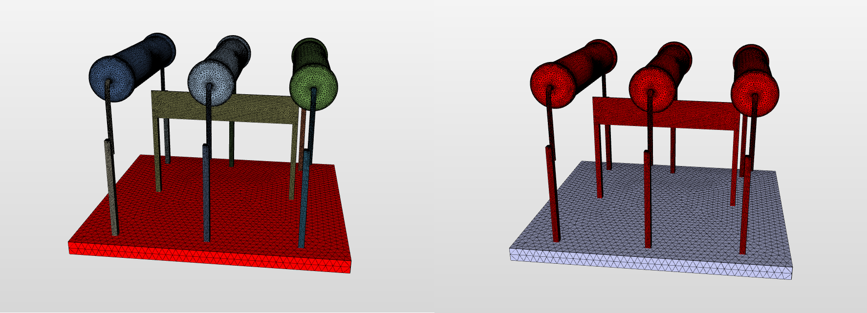
Simplified material assignments for the plate and all resistor components.

Resistor volume heat source and convection boundary condition.
Temperature distribution for a steady-state heat transfer simulation assuming every resistor serves as a 1W heat source.
Best Alex