In this post we will show how to use SimScale online post processor for CFD simulation post processing.
We will use the project “Aerodynamic of F1 Race car”, import the project by clicking at this link. The project contains an incompressible steady state run which will be used for post processing.
Instructions
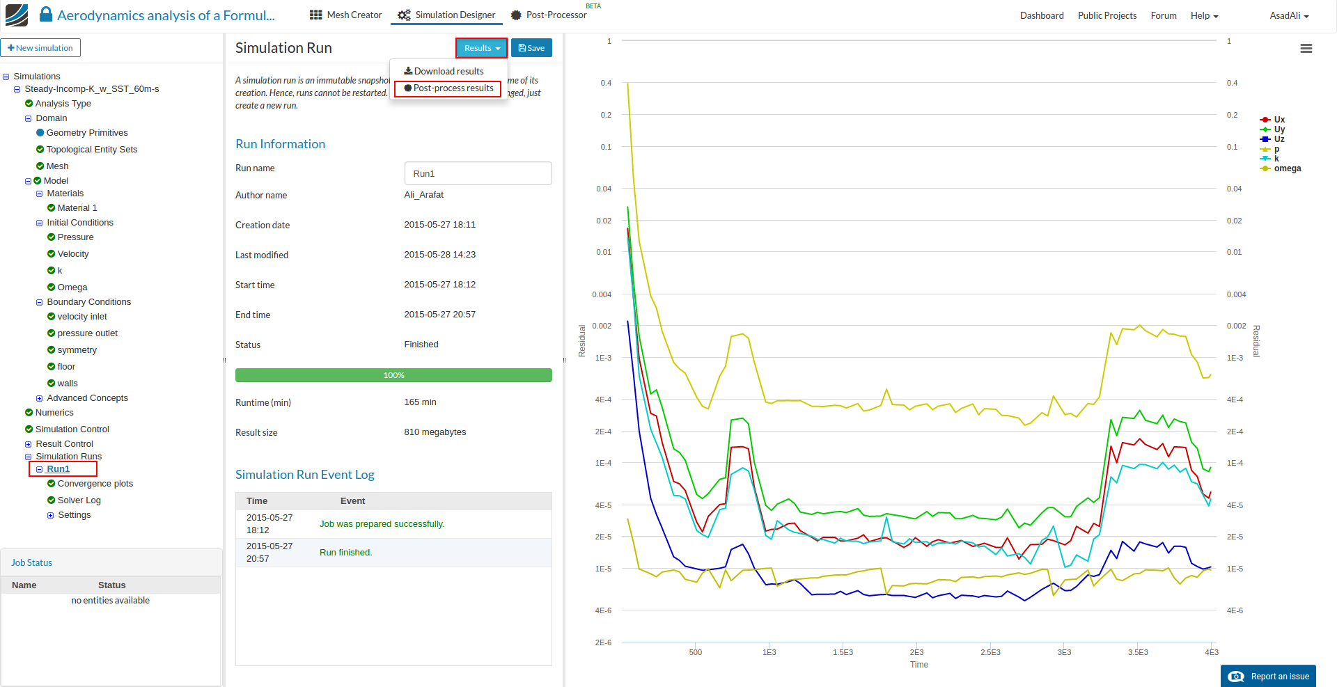
- Once simulation run is finished (the progress bar turns green) then click on the Results and select Post-Process results.
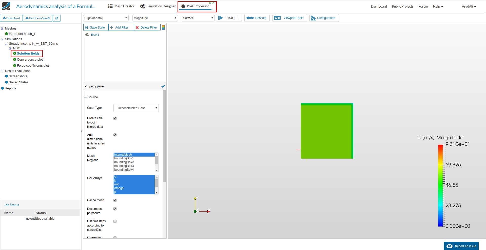
- Immediately you will be moved to the Post-Processor tab. The simulation will be loaded to the post processor in a few seconds (depending on the size of simulation). Once the simulation is loaded make sure simulation is at the last time step.
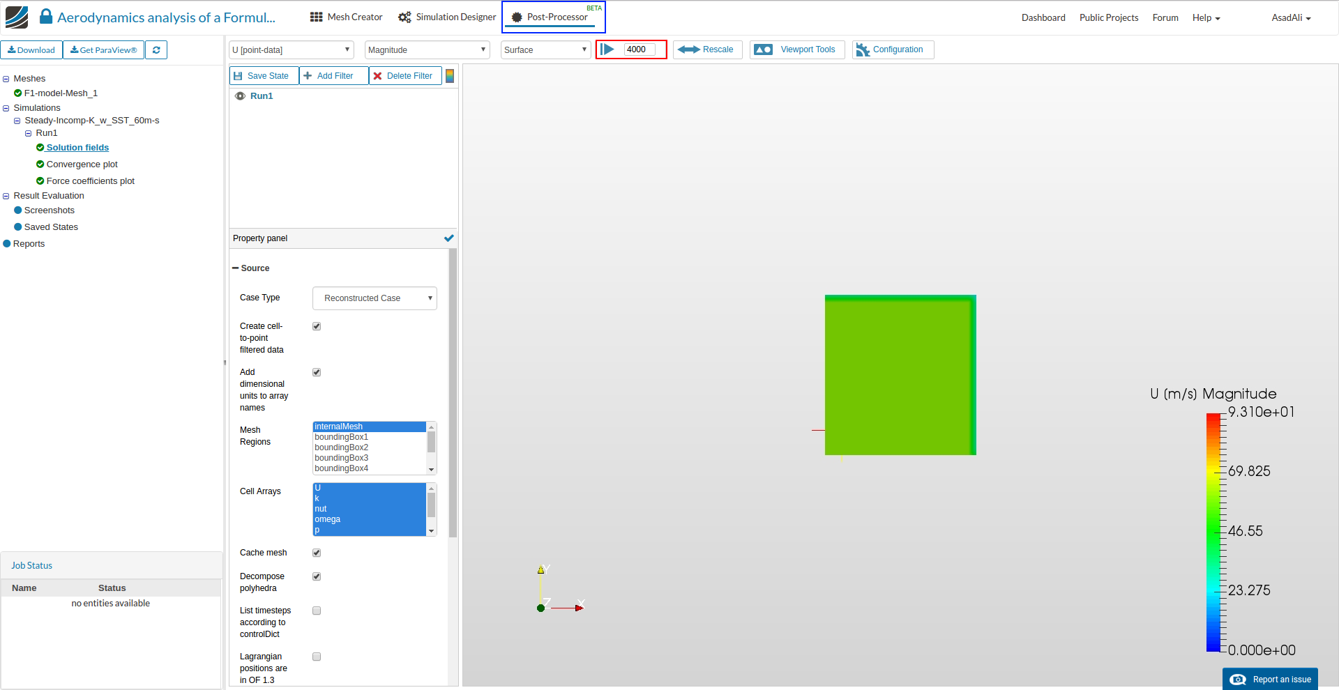
(You can also directly move to the Post Processor and select the Solution field of the simulation you want to post process.)
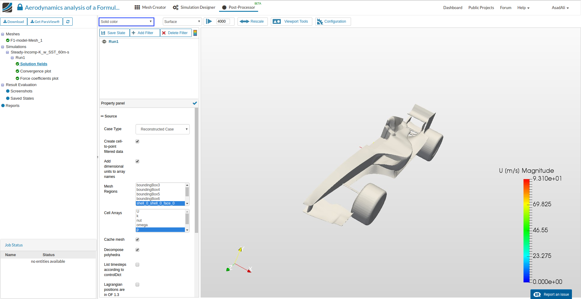
- Now first step is to load the car body to the viewer. In the Mesh Regions select only the car body (select only the model faces). Also in the Cell Arrays select only the p field and save the selection by clicking
 .
.
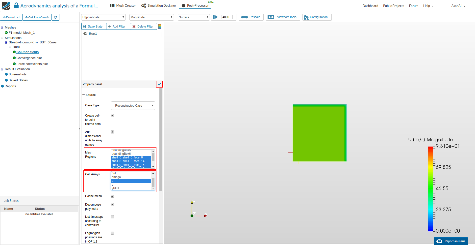
- This way we are just loading the car body with only pressure field into the viewer. Once saved, you will get window as below.
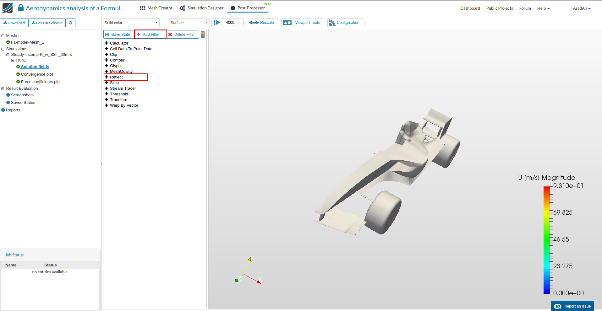
- Next step is to make the full car model by reflecting this half model to the other side. Select the tab Add Filter and select the Reflect filter.
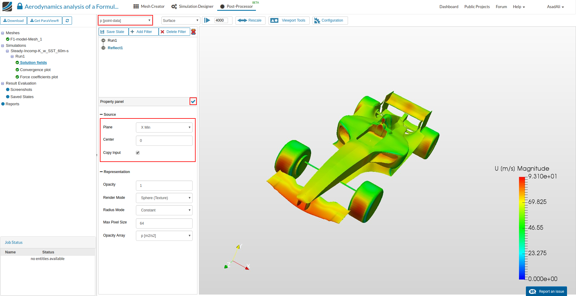
- Set the filter values accordingly and save the selection by clicking . To show the pressure distribution on the model, change the field to p[point data].
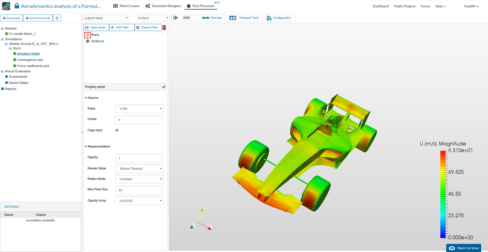
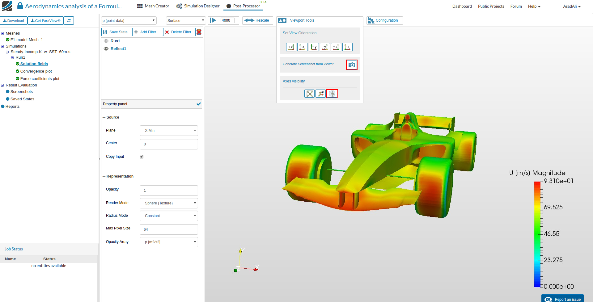
- Now hide the Run1 by clicking the “eye” sign. To save the image of the model at this point go to Viewport Tools and click the button next to “Generate screenshot from viewer”. Also hide the “Rotation point” by click the relevant button. You can also change the orientation of the model here.
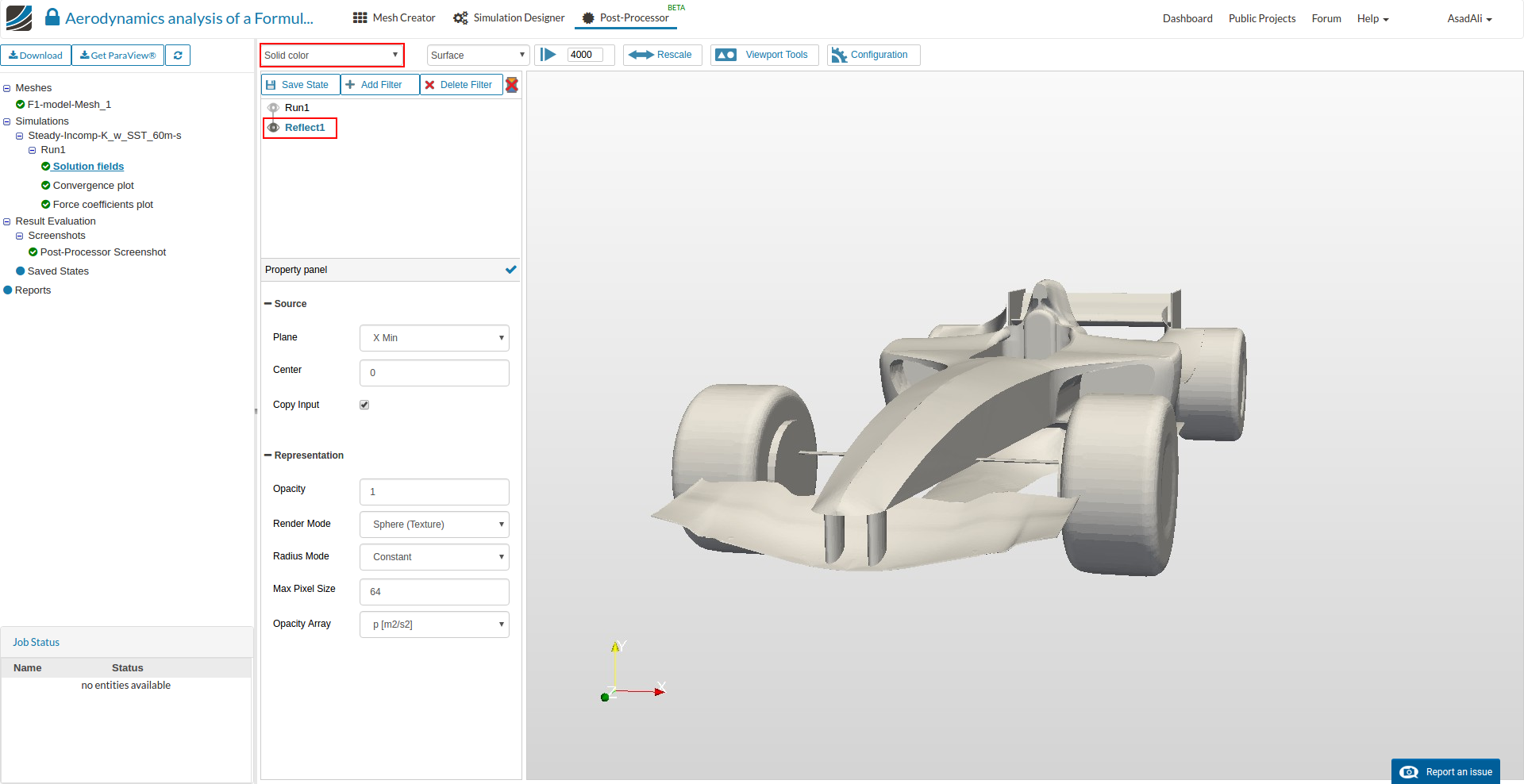
- Now make sure that Reflect1 is selected (highlighted in blue color), and select the Solid color from the fields.
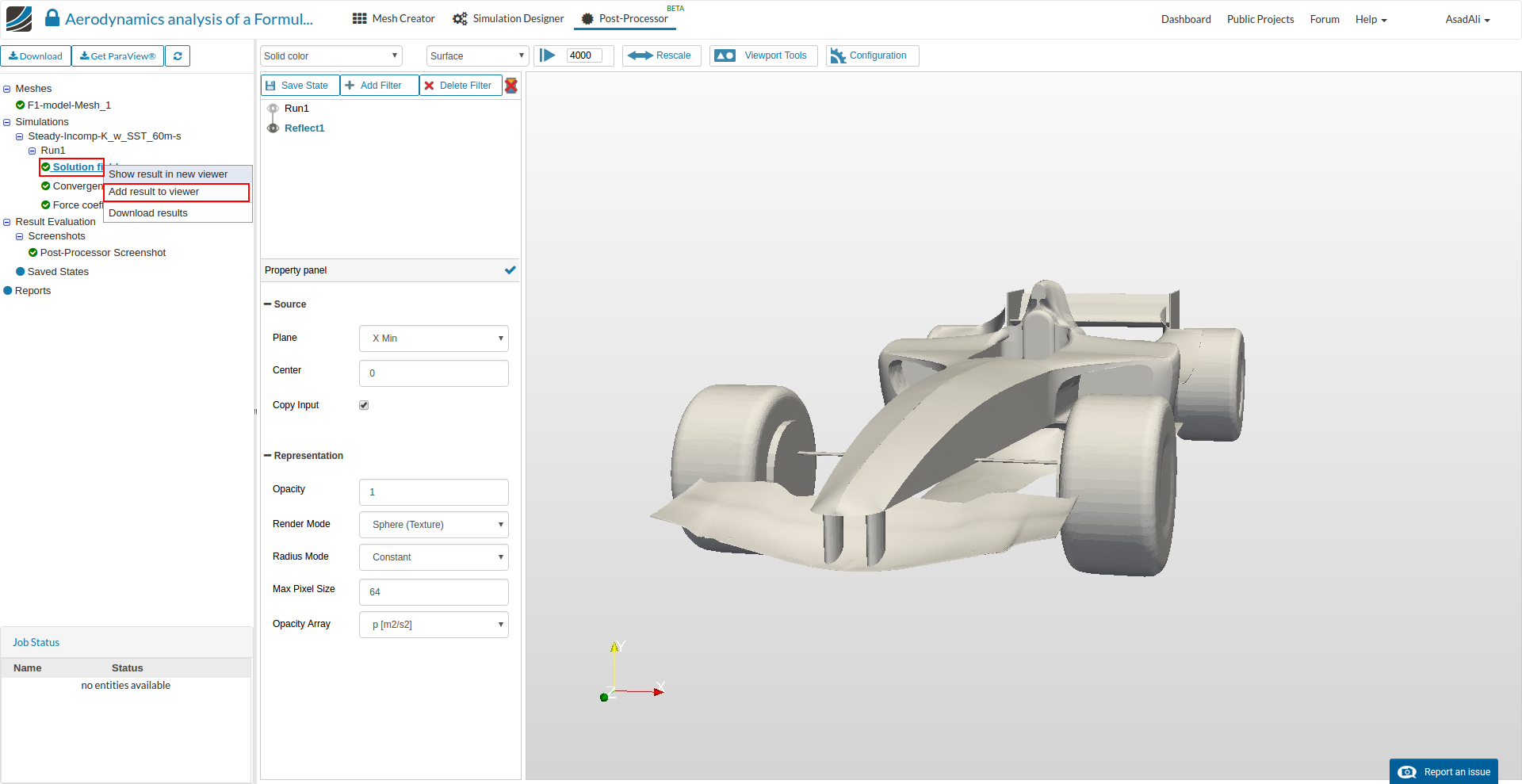
- Now to add streamlines, we have to load the simulation again. Right click on the simulation Solution fields and then click Add results to viewer.
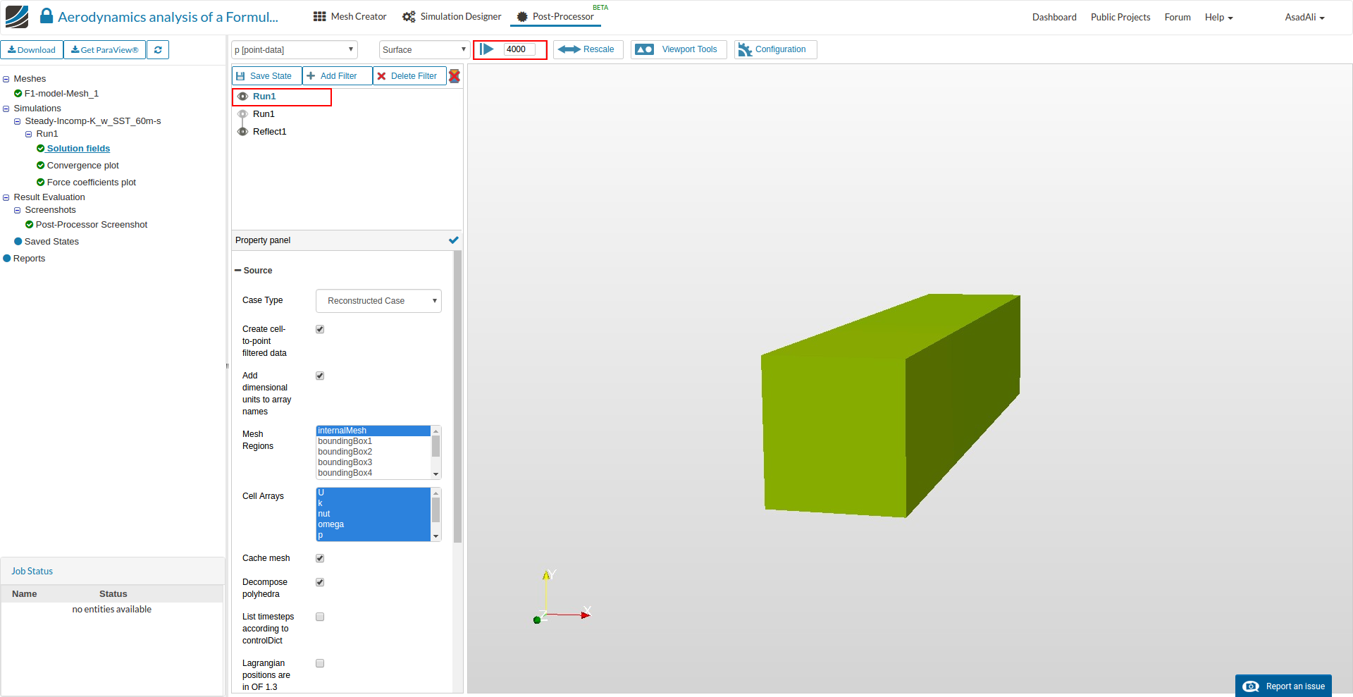
- Now make sure newly added Run1 is selected and and simulation is at last time step.
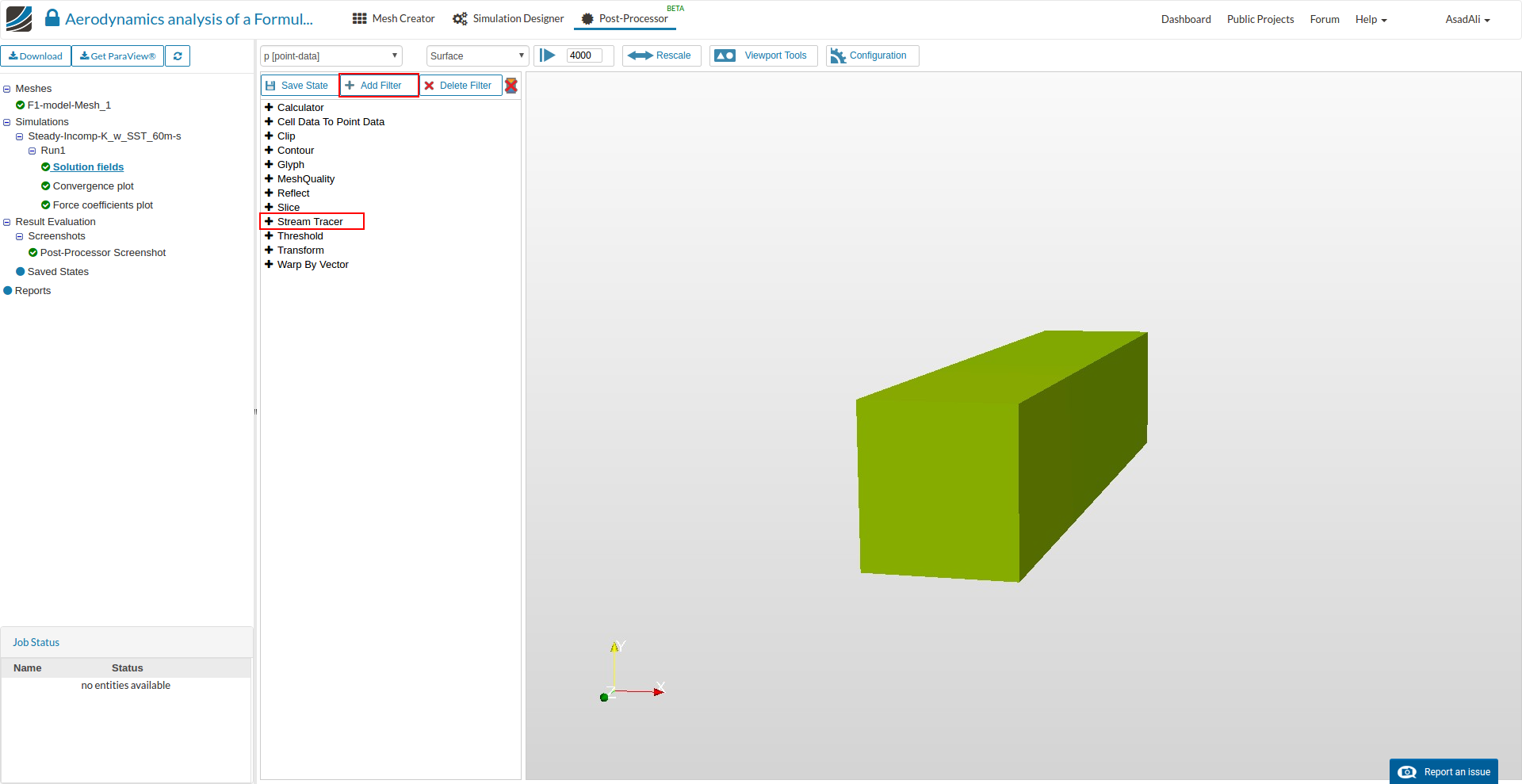
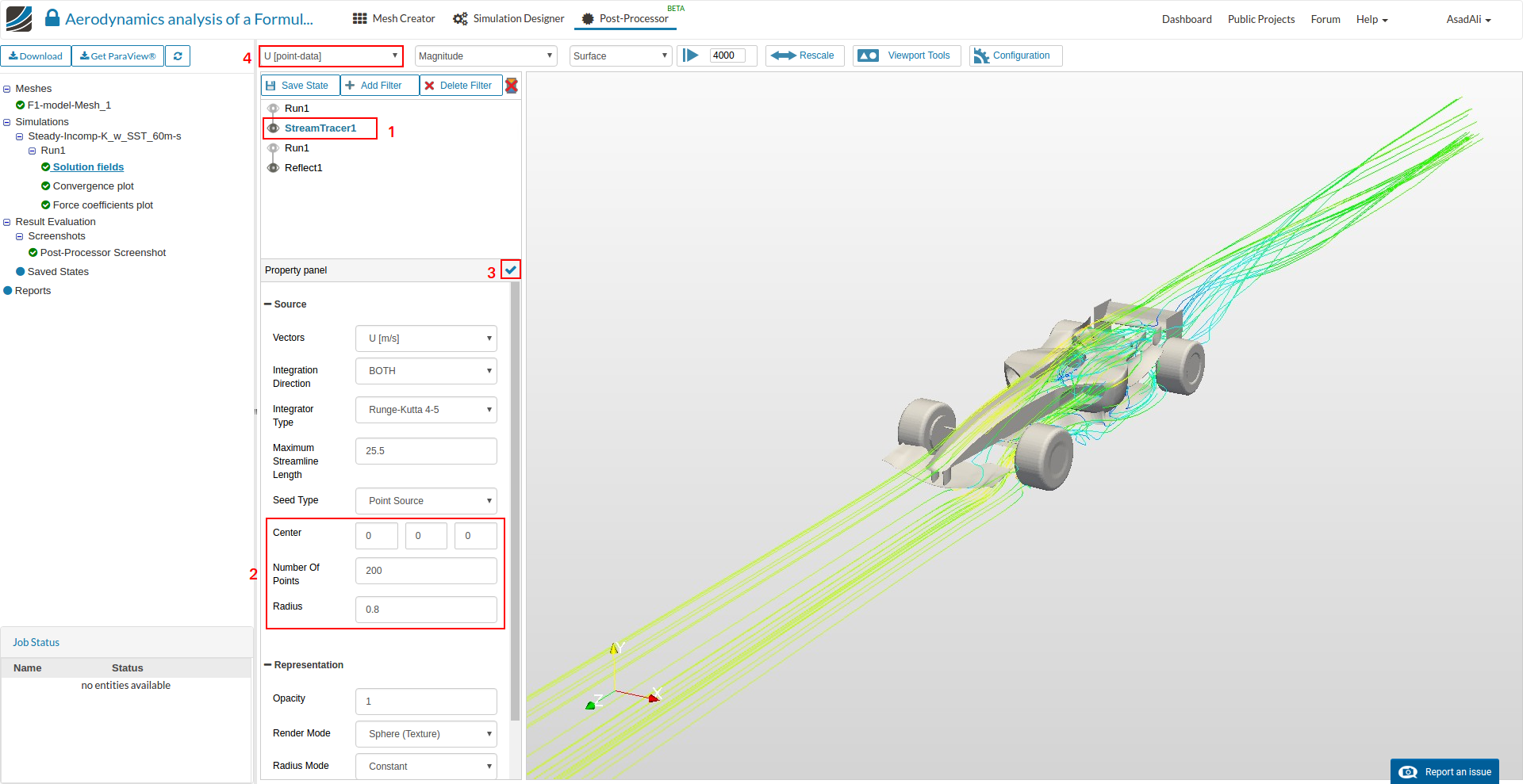
- To add streamlines, while new Run1 is selected, click on the Add Filter and add a filter for Stream Tracer.
- Set the streamline parameters in “Properties panel” accordingly and save the selection. Select velocity field for the streamlines and save the screenshot.
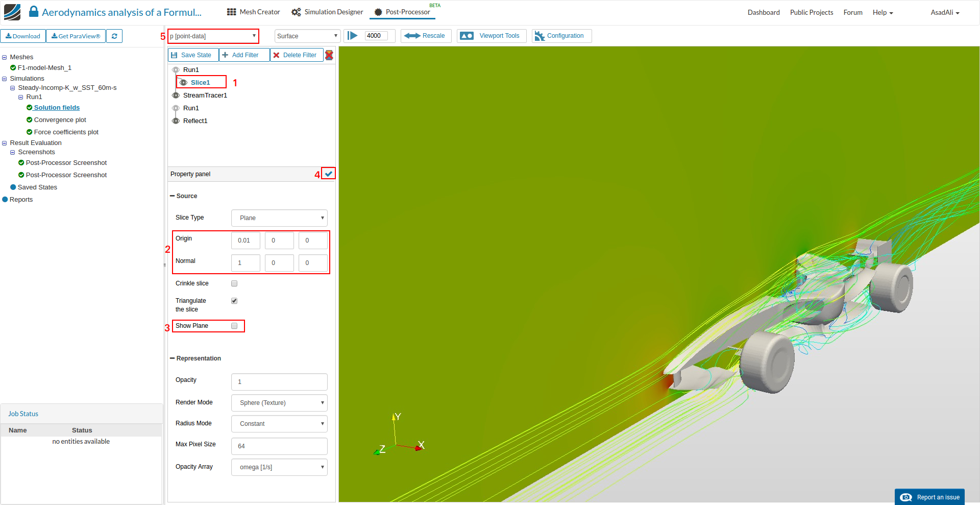
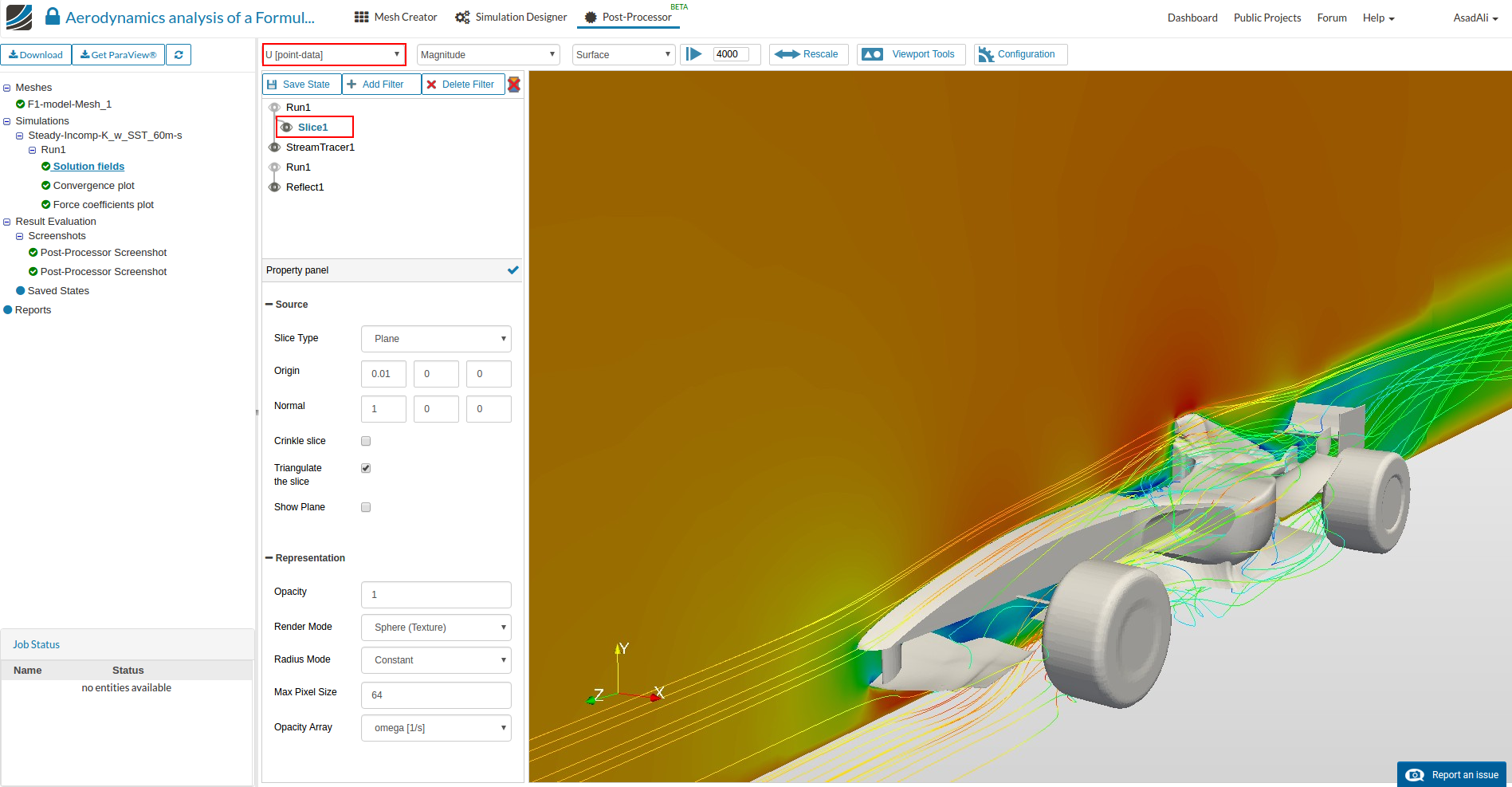
- To add another Slice filter, click on the new Run1 (should be highlighted in blue) and add another filter Slice.
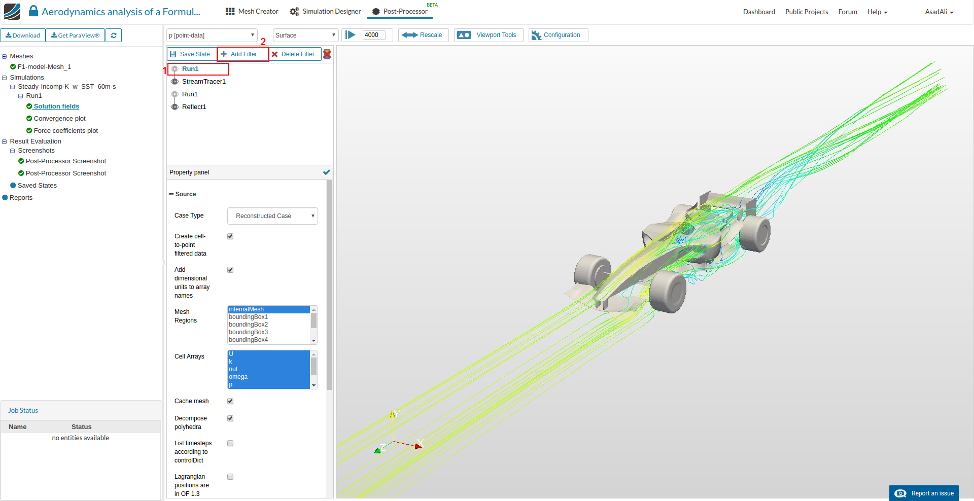
- Set the parameters in “property panel” and save the selection. You can change the plotted field by changing the field to p[point-data]. Make sure streamlines are also visible.
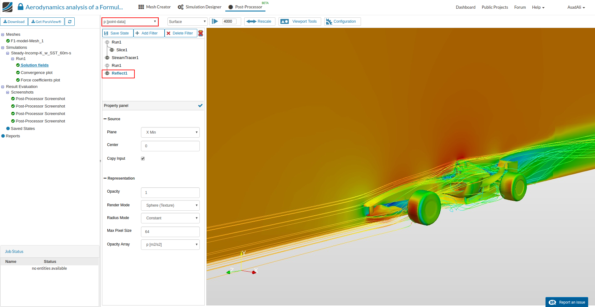
- Now change the plotted field on the slice to the velocity, and field on the car to the pressure by clicking the respective buttons. Save the screenshot.
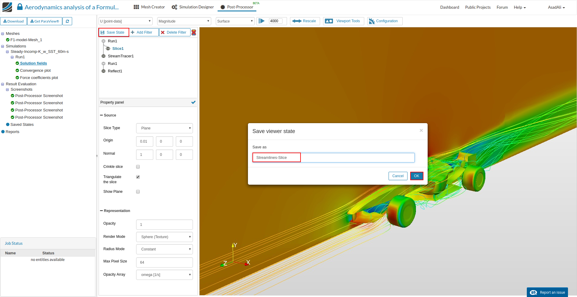
- Now to save the state (for later use) select the Save State, rename and save.
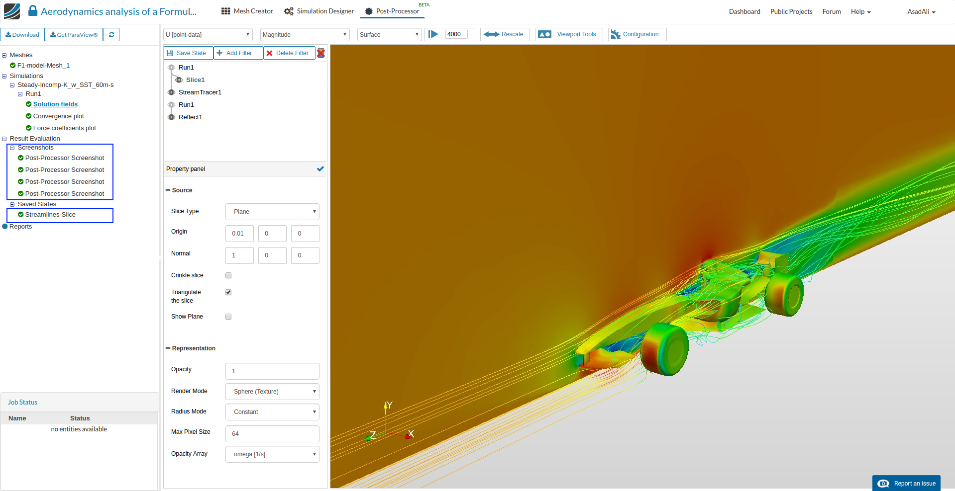
- Saved screenshots and saved states can be found under Result Evaluation and can be viewed any time later.
Notes
- Always make sure the right item is selected in the post processing tree in order to change the properties or to add the filters.
- Use hide (eye) button to hide or view different filters.
- Use “Toggle Colorbar” button, next to the “Delete Filter”, in order to hide or show the colorbar.
- Depending on the type of analysis add more filters and change the properties of the filters e.g origin and normal axis in case of slice.
- Save the screenshots and give them proper names.
