Hi, I have been using the DHeiny butterfly valve example to practise manual meshing and turbulent sim setup.
When I load the project some things don´t make much sense for me (newbie, please enlight me).
First, I don´t see a wall BC set, why is this?.
Second, don´t understand really the outlet BC of the “custom” type and why “inlet-outlet” k-w values are set there.
I would expect an inlet with some stimated k-w values, btw for this shall be used also “custom” BC, shound´nt it?
I tweaked the sim options to use k-e, set walls BC, a “custom” inlet with defined k-e and pressure outlet = 0, but what seems a converged solution doesn´t make much sense either (k is oscillating somewhat).
So I am a bit lost.
great to see you digging deeper into that project! So regarding the BC setup:
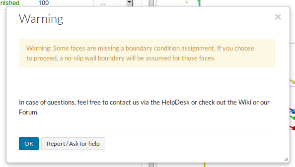
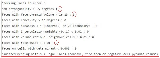
Missing Wall BC: For every boundary of the flow domain, where no Boundary condition has been assigned, SimScale automatically assigns a no-slip wall boundary. You can see this once you create the run, the message below is shown. So the no slip wall BC is used, but you don’t see it explicitly. But now that you are raising this, I think especially for library projects it would make sense to have all boundary conditions explicitly created to make them really visible to avoid confusion. I’ll keep this in mind when creating the next simulations.
Inlet BC: The setup I used is a velocity inlet BC, where turbulent quantities are set as fixed values derived from the initial condition values (velocity inlet documentation). You’re right - if you would like to set the turbulent values explicitly, you could choose a custom BC applying fixed value for velocity, zero Gradient for pressure and fixed values for the turbulent quantities, exactly how you did in your sim
Outlet BC: I could have chosen the pressure outlet, which would be the most simple one (zero gradient for velocity and turbulent quantities as well as a fixed value for the pressure, see pressure outlet documentation). However as the flow domain downstream of the valve is quite short (actually I would say it’s too short) I suspected potential backflows, I decided to go with an inlet-outlet BC for the turbulent quantities. They basically switch between a zero gradient and a fixed value BC depending on the velocity direction. This means if a partial backflow appears at the outlet, for these cells a fixed value for the turbulent quantities is applied (this is why there are turbulent values given) which makes the simulation more stable.
I briefly checked on your simulation setup and in general it looks good to me - the BC setup makes sense! A couple of points, that might be the reason for the convergence behavior you’re seeing:
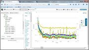
Transient effects: During the project setup I also ran a quick transient analysis of it and behind the valve, there appears a flow separation that creates a transient flow pattern, that can not be covered correctly by a steady-state solver, which could lead to the residuals not going down. This gif shows a bit what I mean:
Turbulent initialization: You’re using different values for k and epsilon in your inlet BC than your initial conditions. Is this on purpose? However I think that should probably not be the reason as this might only lead to a slower convergence but not to the oscillating behavior you’re seeing.
Mesh: Especially the edge before and after the valve are sensible to the layer inflation. It seems not to be well meshed in that area. How about increasing the refinement level of your region refinement a bit more there? (The one with the sphere)
Flow domain: The flow domain is too short as the downstream flow interacts too much with the outlet patch. I used this project in a webinar a couple of weeks ago (video is here) where I extruded the flow domain more.
@gholami, @jprobst, @Maciek - did I forget/overlooked something? Maybe you have another hint?
You’re welcome! I forgot to mention: If you’re looking into this kind of simulation, I recommend checking out this validation study of a butterfly valve flow simulation that @Ali_Arafat put together (see image below). It compares the simulation results of SimScale with experimental data from a research paper. The complete project can be imported via this link:
As I was called to the blackboard I’d like to write a few words about this simulation – just needed to check something first.
IN SHORT
In my opinion this simulation is feasible in its current geometry configuration. It’s true the domain is very tight and there is very little room for the wake behind the valve, but still it can converge. Please, give me a couple of days to sit on it, ok?
YOUR SIMULATION
Beginner or not you shouldn’t send us things like this:
You could turn the blind eye on non-orthogonal element – despite we don’t know the extent of this deformation – but two other errors disqualify the mesh. I know there are only 8 of them, but we don’t know their location. So you should generate the faultless mesh and then proceed with your simulation.
It’s true that in every day practice there are situations where you have no choice but accept low quality mesh. Sometimes you have very complex or specific geometry and obtaining good quality cells in the difficult regions is simply beyond mesher capabilities. But for your own good you cannot simulate with invalid meshes.
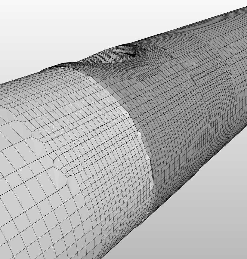
Further, please take a closer look at your boundary layer too (!).
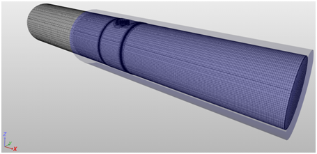
VALVE
I would say this simulation is a kind of provocation. It’s something to encourage you to try simulating, to investigate the problem and play with the settings. Definitely it’s not a solution given to you on a plate.
Why? Let’s look at the domain size and the velocity. The pipe section is roughly 0.5 [m] long and its diameter is 82.9 [mm]. The flow velocity is set at 0.5 [m/s]. Multiplying size by speed we get about 2.7 [l/s] (litre per second). It’s a pretty good speed I would say.
Now we go to Simulation Control / Time step length and the step is set at 1 [s]. How can you expect it to stabilise when the time step nearly doubles the domain length? Also total time was set at over 27 minutes. It has no sense to me.
I think I’ve written about it previously (@sjoshi topic I guess), but I’ll do it again. Imagine yourself a particle of water travelling from the domain inlet to the outlet. If you want to study its way carefully you have to divide the path it goes into sections (steps) and you do it by setting a ‘time step’. The more steps (but not too much) the better view of particle’s path you will get. So in this case, when your time step is about twice as big as the domain length it’s difficult to expect that solver will predict or recreate particle’s path properly.
How to do it in SimScale? Well, I have an idea that I know it works and I’m currently trying to check it out with different numerical settings I’ll let you know if I had some positive news.
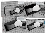
This is a comparison view of the 3 meshes, auto coarse, auto fine and manual.
All snappyHex.
Actually the auto results (coarse and fine) seems better looking than the manual, and give no bad cells in the log.
I just was trying the manual for the first time.
Seeing the result of the auto-fine I think that maybe the initial mesh for manual was too coarse. The refinements that appear in the corners seems to difficult the overall mesh coherence, more than helping.
How can that be controlled? I did not activate the surface features refinement.
I don´t get how to configure the BL controls to get a continuos prism layer that does not collapse at the corners. It also has some “jumps” maybe due to the abrupt changes in refinement levels, what do you think?
I used, a region refinement near the valve, surface refinement in the butterfly and the BL creation. What do you suggest to improve, tweaking the parameters of current sets, or do you think that is it needed more detailed refinement regions/surfaces?
How can be detected where the zones with the problematic cells are?
Regarding the time steps, note that the sim is steady state, and the info I got is that in this case it doesn´t matter the timestep value, just the number of steps to allow the solver to converge.
Hey @rarrese, yes I’ve seen your meshes and that’s why I mentioned them in my previous post.
For me so far the best approach to mesh geometry for CFD cases is snappyHexMesh which means manual settings of the most important parameters. In fact you don’t have to change a lot and all I do is:
BOUNDARY LAYER
I set _BaseMeshBox parameters – obvious
I change Feature Angle and slip Feature Angle from 60 to 350 – as far
as I understand it it’s an opening angle of two surfaces sharing a
common edge.
I know @dheiny wrote in one of my topics that it’s far enough to increase Feature Angle up to 180 degrees, but as far as I’ve noticed it may not be. Further, David suggests we should change only the first value, but when I leave slip Feature Angle at 60 there is no response from the mesher and BL cells are still inappropriate. Anyway at the moment setting both features at the same value works the best for me.
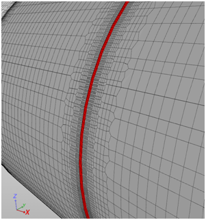
Two strange behaviours of BL you see are: stair stepping (disappearing cells) and layer compression (cells’ squeezing). These features are to help mesher cope with difficult regions, where extruding even a single cell of BL is problematic. Additionally, in relative meshing, compression is / may be a result of base element size. I’m afraid we have to accept BL’s lack of continuity in some areas. Just try to check your mesh carefully.
Topic about relative meshing:
I also increase nSmoothSurfaceNormals from 1 to 3
REFINEMENTS
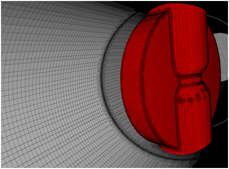
I did only one region refinement here. The valve area and the wake behind it – you forgot the wake is what causes the convergence problem in this case.
And don’t ask me why there are these patches of additionally refined mesh on valve’s surface. I guess there must be something slightly different with geometry surface there and hence this unexpected behaviour.
I avoid using Feature Refinement (edge refinement) as it often causes me troubles. I think a bit more effort with manual surface refinement is better approach and gives me greater control over the mesh.
INVALID CELLS DETECTION
I’m afraid at this stage there is no such possibility. But you are absolutely right and it would make our life easier if there was a tool which could highlight invalid elements. @dheiny what do you think? Is it feasible in the near future?
TIME STEPS
Well, I’m a bit confused here – the labelling is clear to me. In other programs, regardless of steady or transient state, you still set the time step and it does have an influence on simulation run…
SIMULATION
I’ve tried the valve already and after a few attempts I went back and started with more simple case – to reduce the number of elements and time needed for experiments. So far I was able to achieve expected convergence in a steady state for both k-e and k-w models. (I just don’t control it fully ) And it seems to me that we have to switch to epsilon (which I don’t like) as I’m unable to reach minimum Y+ values for omega. – Everything points at very dens mesh here. In such situation we won’t be able to provide required first cell height.
Ok, that’s it for now. I continue my experiments and I’ll let you know the results and conclusions.
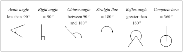
I have some doubts understandig the “feature angle” concept, just to check if I understood:
base snnappy Hex parameters: resolve feature angle (30º by default)
I understand: if angle between normals of body surfaces >30º refine in that area to max. level.
Layer mesh: feature angle (60º by default) “Angle above which surface is not extruded”
I understand: if angle between normals of body surfaces >60º then “collapse” the layer there.
What is the physical sense of terminating the BL mesh in this features?
if 60º by defatul I assume that it is because of some good reason.
BTW with 180º in this parameter and extending the region refinement I could pass with 0 errors the quality checks.
Regarding using k-e or k-w SST.
For k-e it is needed to check y+ value of first cell, and I assume that also that BL full height is resolved inside the prism layer, doesnn´t it? For y+ value can be done a initial guess, but for height of BL refinement (i.e. select nº of layers and grow factor), is there any thumb rule for a first guess?
For k-w SST y+ value has to be very low. <1-5 depending on objective as far as I could find.
The ley point is to resolve the BL in detail with enough cells.
As previously asked, how to get a initial guess for BL full height to define number of layers?
What does it mean the possibility of selecting “wall functions” with SST?
I understood that the full point of k-w SST advantage is resolving the BL area so it gets a more realistic model, so don´t see what use has selecting wall functions there, maybe for zones where is not possible to get y+ low enough?
I’ll need to check on your project again in more detail, @rarrese before I answer on some of your questions. But to provide some first comments:
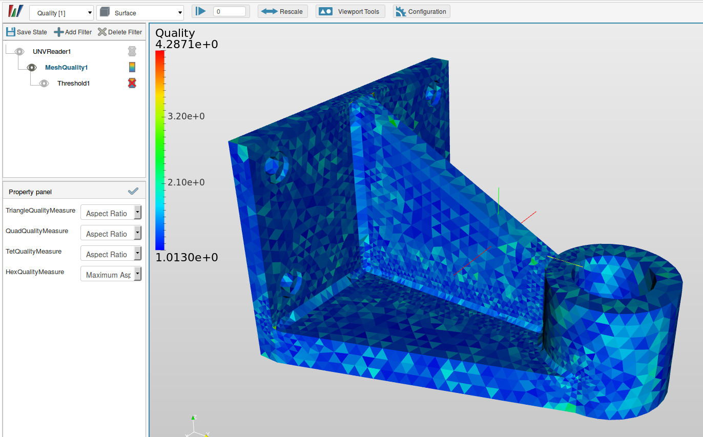
So there is already an option in the post-processor to check on element quality of a mesh prior to simulation. However this method only checks on hexes and tets in a volume mesh as well as tris and quads in a surface mesh (see below images of a tet mesh). As snappyHexMesh creates arbitrary polyhedral cells, this does only provide certain insights into the quality of such a hex-dominant mesh, so it’s not the solution for this.
For snappyHexMesh meshes, I also tend to check the meshing log carefully and tweak the settings accordingly. Most of the time a visual check of the surface mesh shows where more refinements/different settings are needed. Once it seems okay, I run a very simple first run with it (sometimes even laminar) and check on the solution fields. If peak values for pressure and velocity appear, I use the threshold filter to see where they are and if there are bad cells. @Maciek: A method to localize ill formed polyhedral cells is in the backlog and should appear soon.
For the steady-state setup: Indeed, it’s a quasi-static approach, so only the iteration count is important, not the absolute value of the time step / simulated time.
I’ll get back with some more comments, once I checked on the project in more detail.
