Recording

Introduction
Cardiovascular stents are commonly used in angioplasty in order to treat coronary heart disease. A stent is a small mesh tube that’s used to treat narrow or weak arteries. They are expanded in the heart artery to remove the plaque thus allowing for smooth blood flow. The video below shows the basic technique of treating coronary heart disease.

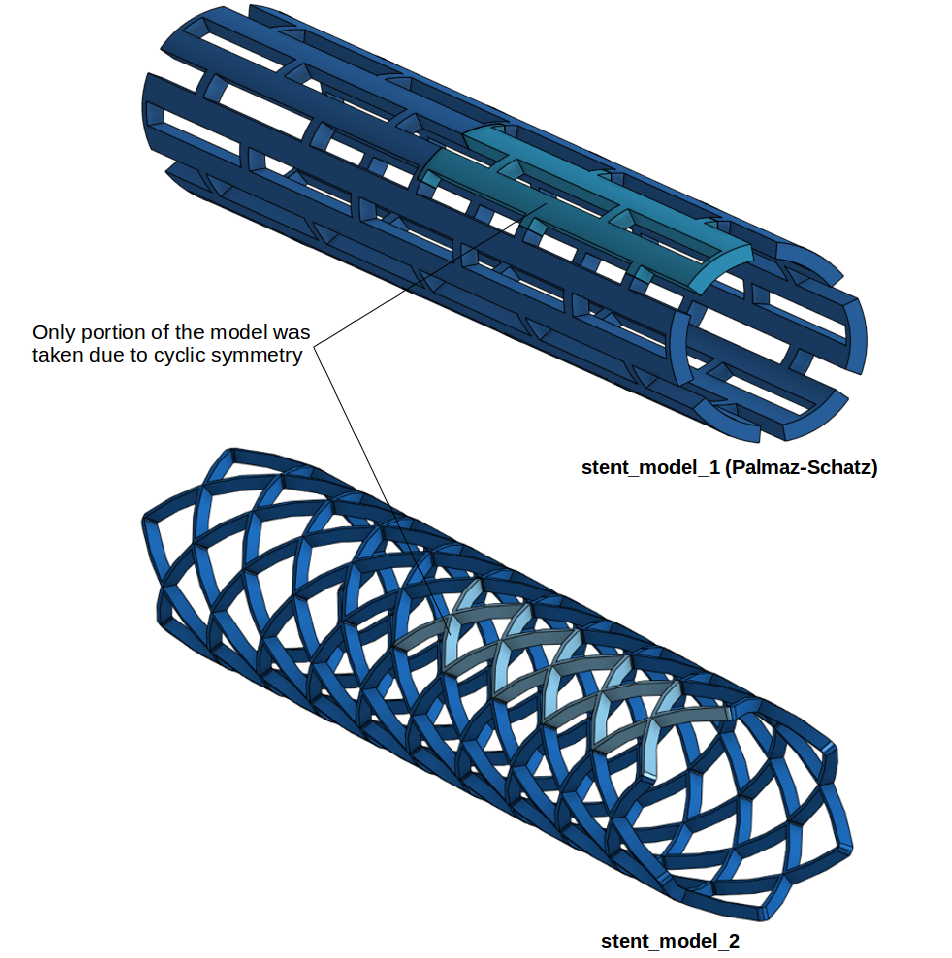
This exercise focuses on the the testing of two different types of cardiovascular stent models (shown in the figure below). The aim is to see which stent type and material is best for treatment.
For simplicity, free expansion of the stents will be performed without the effect of plaque and artery stiffness. Due to cyclic symmetry only a portion of a geometry will be considered. This will help us to do the analysis on a smaller mesh which will require less computational time and power.
The different combinations for performing the simulations are:
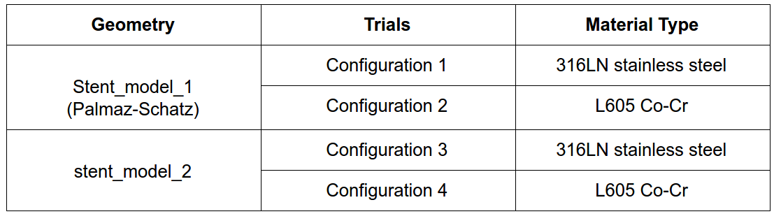
To start this exercise, please import the project into your workspace by clicking on the link below:
Mesh Generation
In the Mesh Creator tab, click on the geometry stent_model_1
Then, click on New Mesh button in the options panel.
Select Tet-dominant
- Element sizing Manual
- Specify the maximum and minimum edge length to be 0.00004 and 0.00003 respectively
- Mesh grading 3-Moderate
- Element order Second order
- Number of computing cores 4
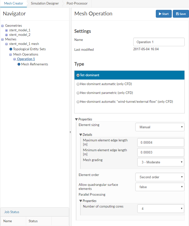
Click on Save and then Start to start the meshing job. The meshing job will take a few minutes to finish and show the status as Finished once done.
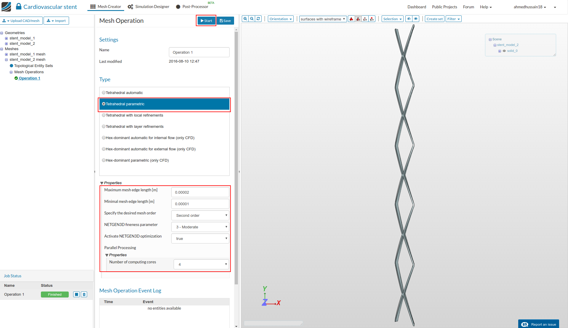
Next, to create a New Mesh for stent_model_2, click on the geometry stent_model_2
Then, click on New Mesh button in the options panel.
- Element sizing Manual
- Specify the maximum and minimum edge length to be 0.00002 and 0.00001 respectively
- Mesh grading 3-Moderate
- Element order Second order
- Number of computing cores 4
Click Start to start the second meshing job. After few minutes the meshing job will finish.
Simulation Setup
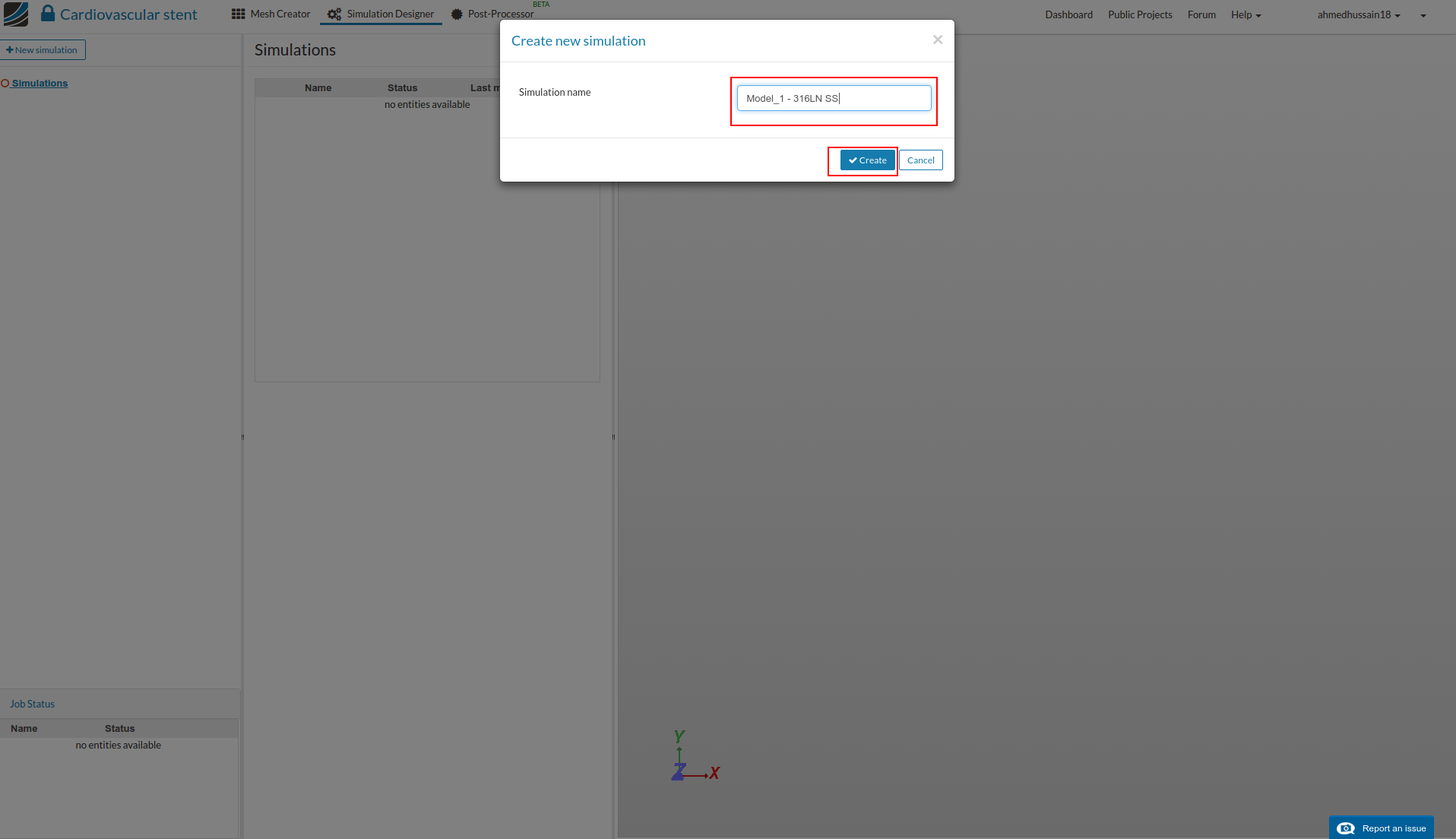
For setting up the simulation switch to the Simulation Designer tab and click +New to create new simulation.
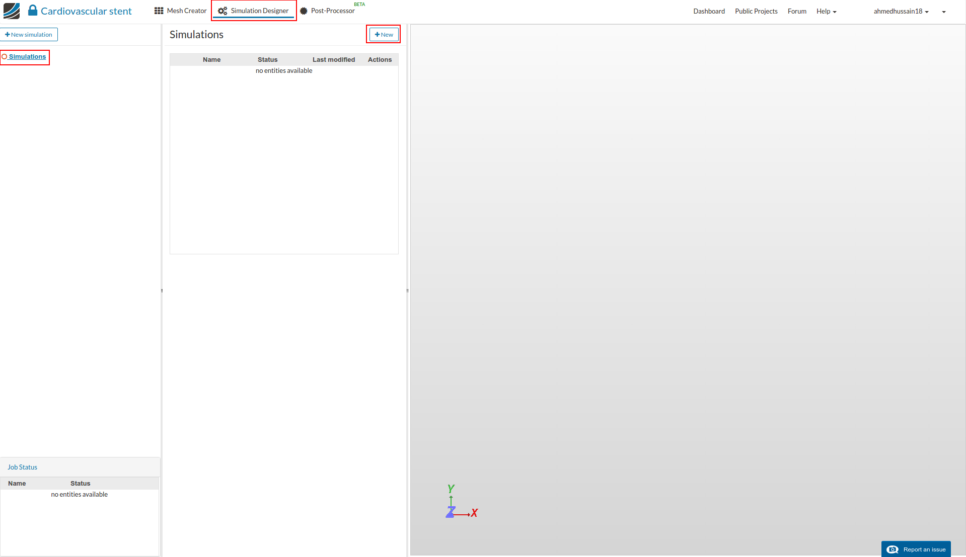
A pop-up will appear. Give the project a name (optional) e.g. Model_1 - 316LN SS in this case and click Create.
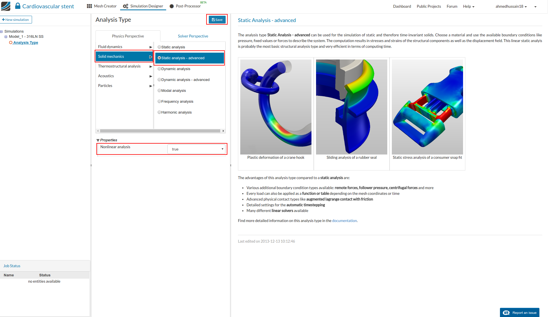
Since our load will be static and deformation will be large including material nonlinearity, select the analysis type Static analysis - advanced under Solid mechanics. Change the Nonlinear analysis setting to true and click Save.
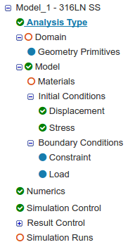
After saving, the Navigator now looks as shown below. Here the entries in red must be completed.
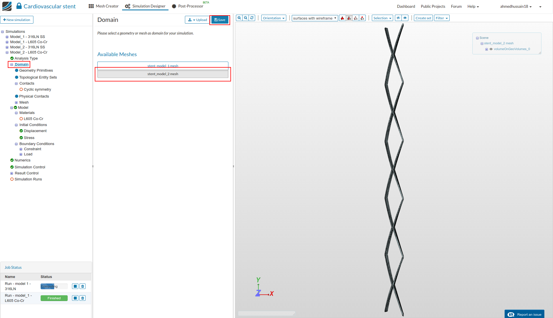
Click on the Domain item in the Navigator and select the first mesh that you created. Click Save. The mesh will then automatically load in the viewer.
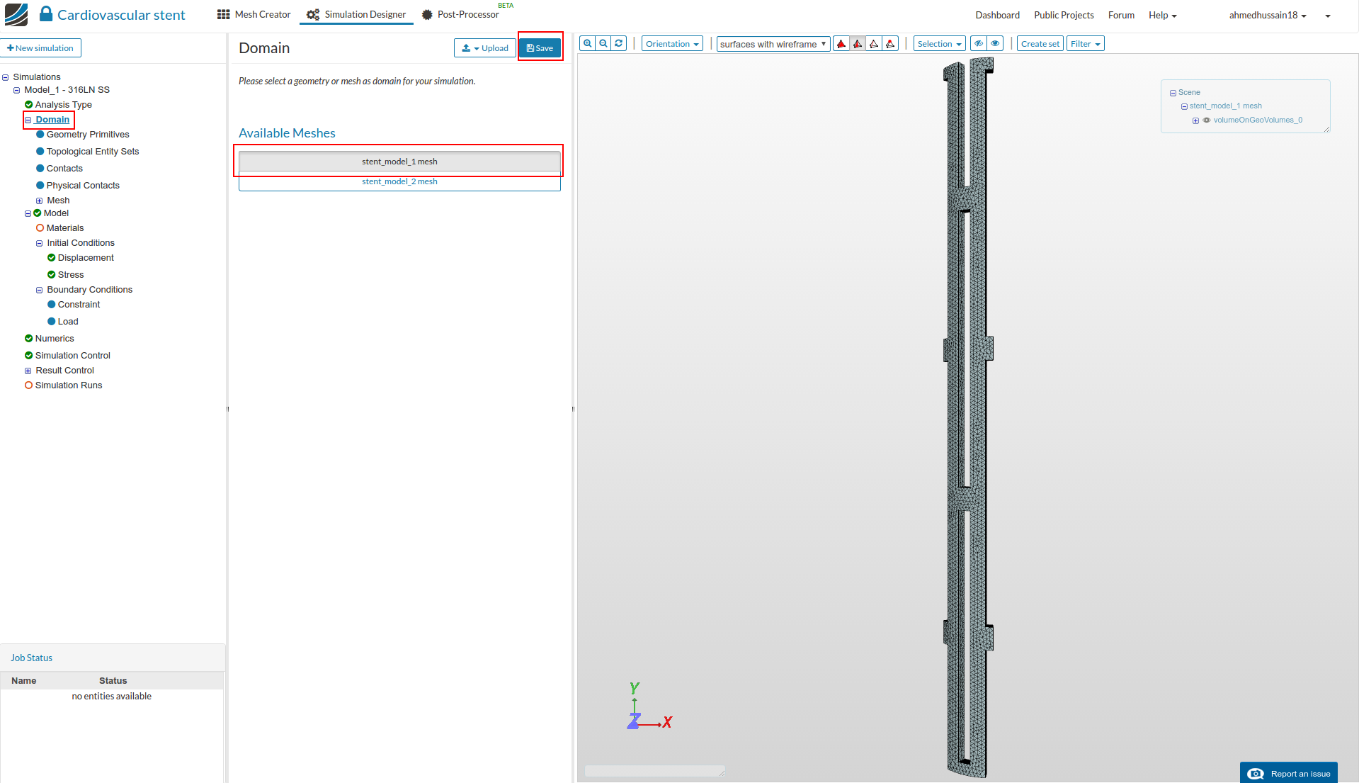
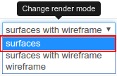
Next change the render mode to Surfaces in the top viewer bar to interact with the mesh more easily.
We will create topological entity sets to make things easier later when we are setting up our boundary conditions. The topological entity sets will be based on the figure below which explains all the boundary and loading conditions.
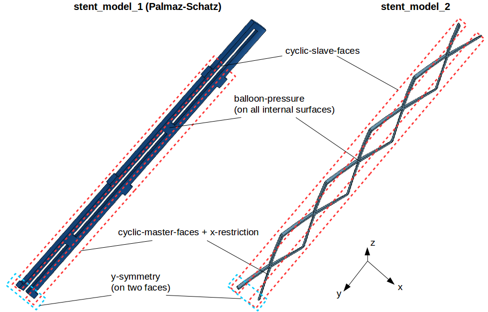
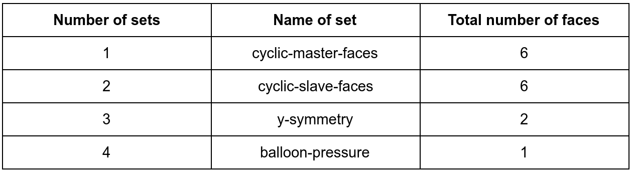
We will create total of 4 topological entity sets as shown below:
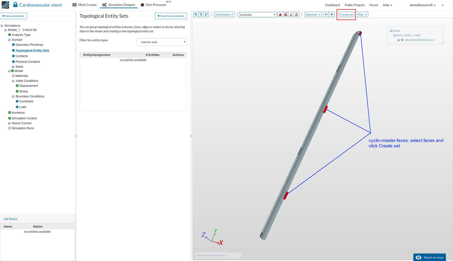
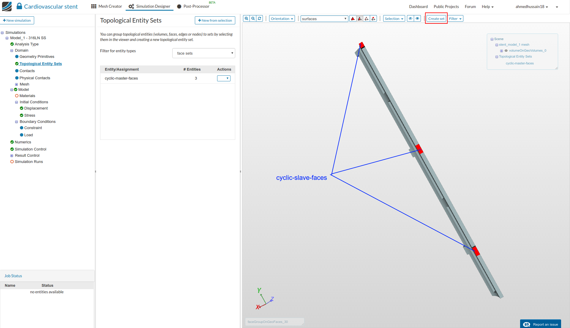
cyclic-master-faces
Click on the faces on the right side of the geometry as shown in the figure below and then click Create set in the top viewer bar. Give the set a reasonable name e.g. cyclic-master-faces and click Create to create the set.
cyclic-slave-faces
Follow the same steps as above but this time select the faces on the left side of the geometry as shown in the figure below. Give the set a reasonable name e.g. cyclic-slave-faces and click Create to create the set.
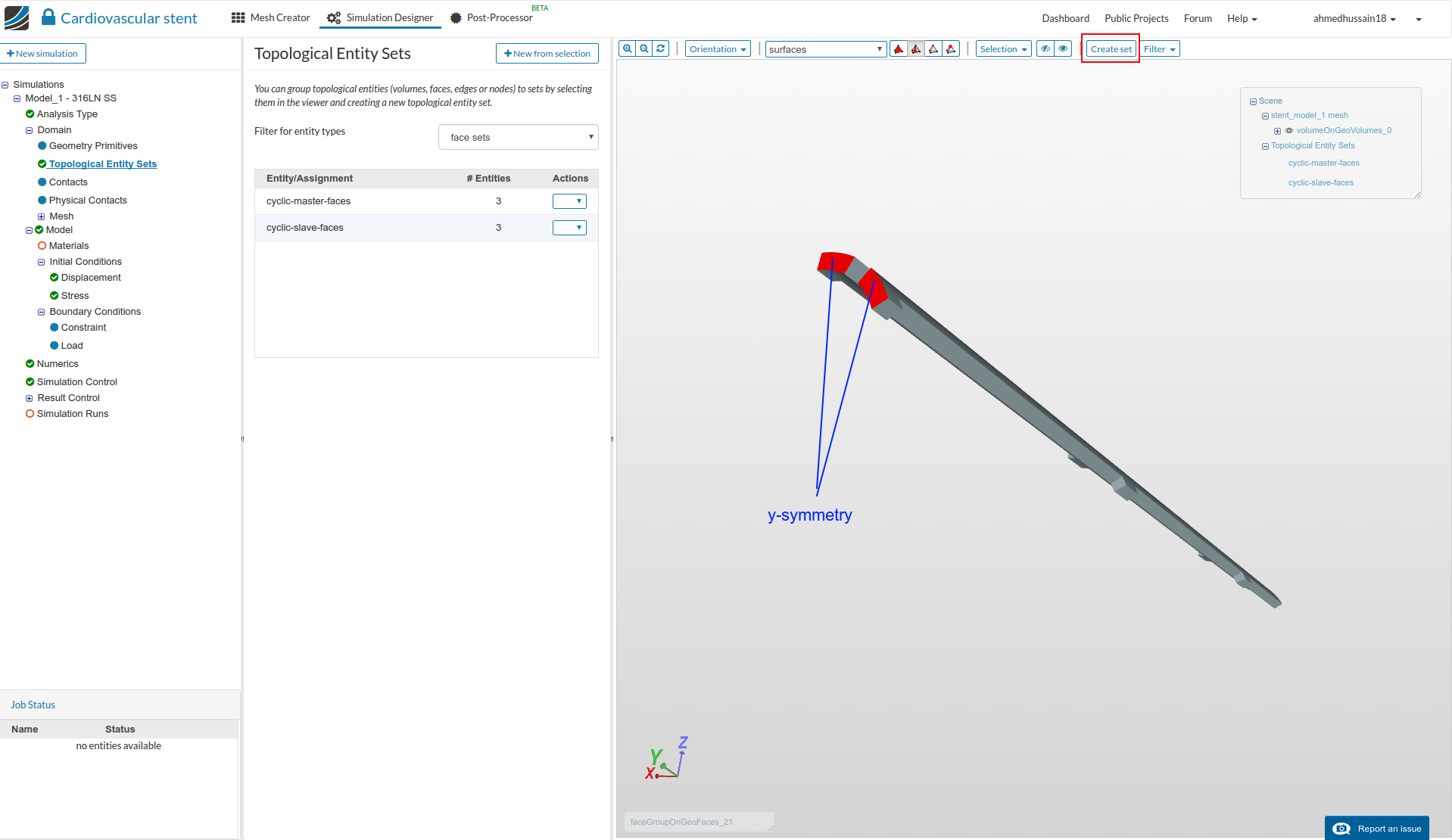
y-symmetry
Following the same steps as above, this time select the upper two faces of the geometry as shown in the figure below. Give the set a reasonable name e.g. y-symmetry and click Create to create the set.
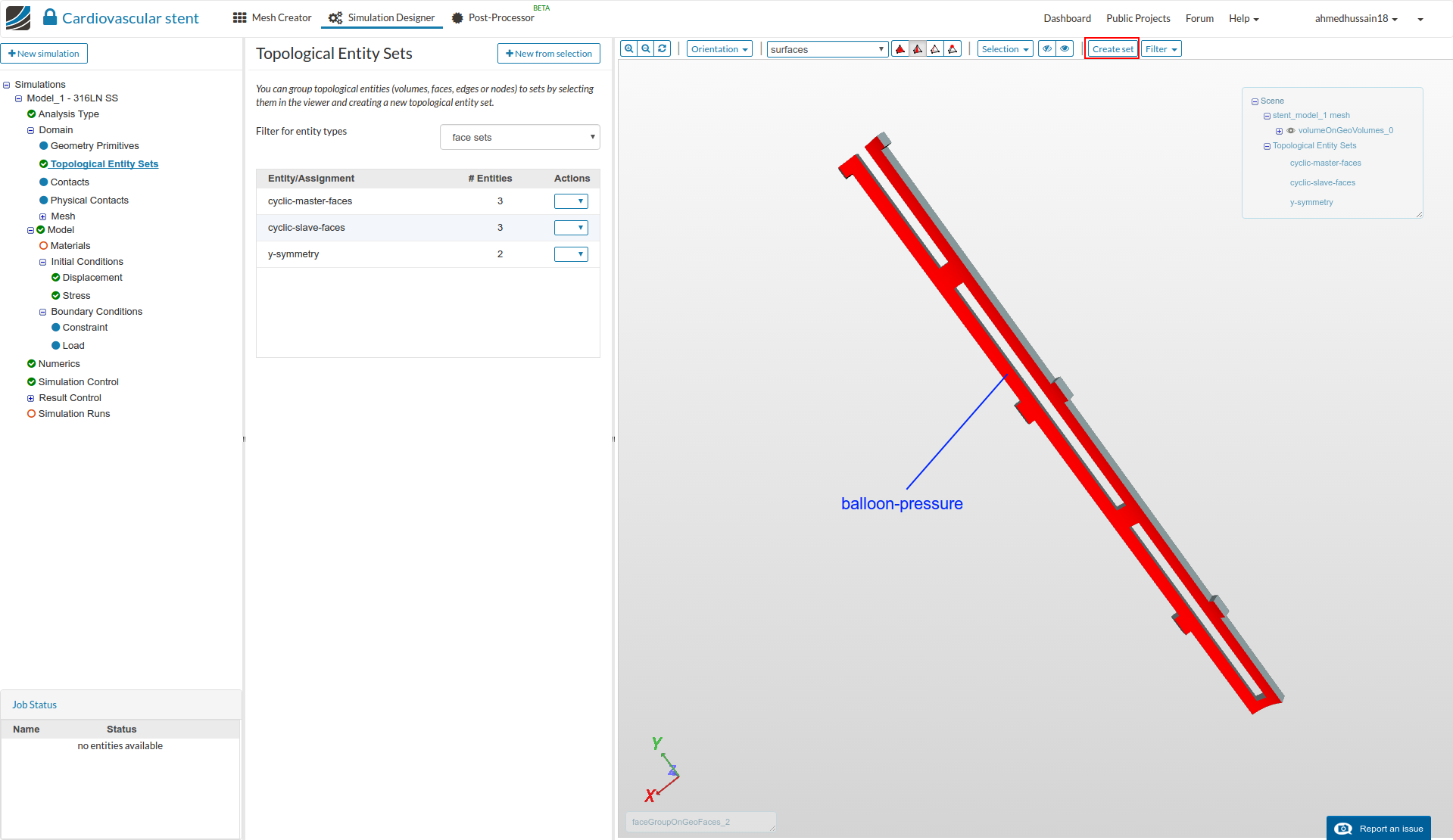
balloon-pressure
For the last set, select the inner face of the geometry as shown in the figure below. Give the set a reasonable name e.g.balloon-pressure and click Create to create the set.
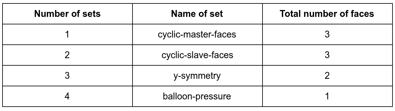
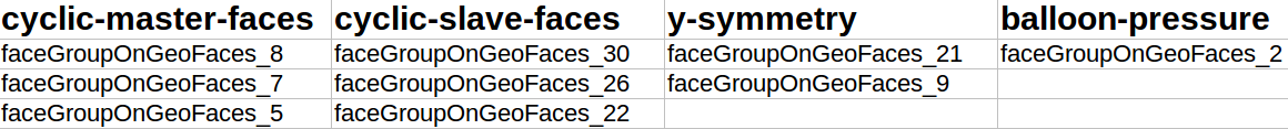
The table below shows the number of faces selected for each topological entity set:
Once the topological entity sets definition is done, we will proceed to define the cyclic symmetry which we require since we have taken only a portion of our geometry. For more information on cyclic symmetry, please see the Cyclic symmetry documentation
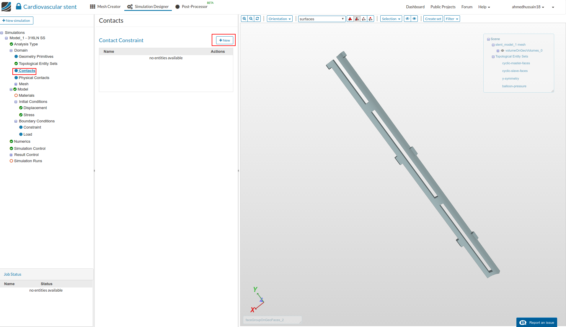
Go to Contacts in the Navigator and click +New to create a new contact definition.
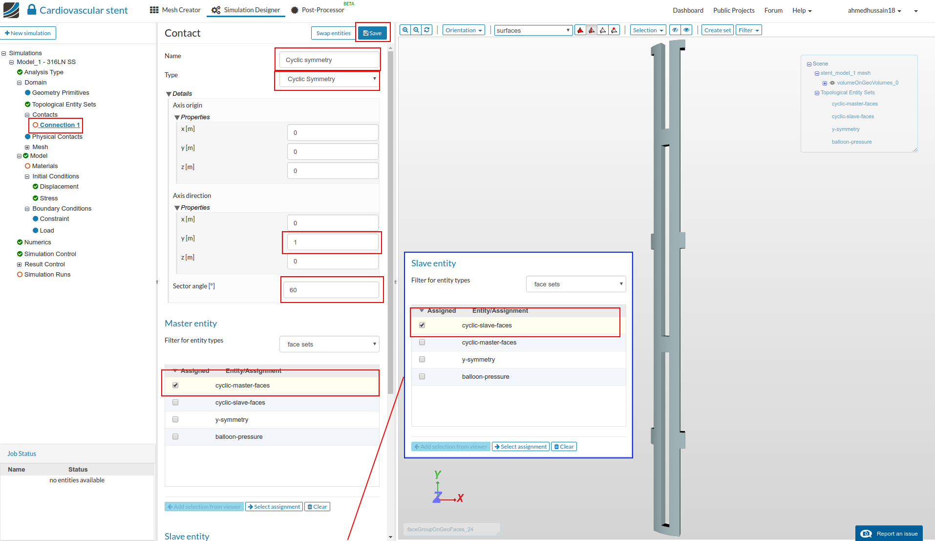
Rename the newly created contact to Cyclic symmetry (optional). Change the Type to Cyclic symmetry. The cyclic symmetry is represented by a right hand rule such that slave surfaces are mapped to master surfaces. Therefore, we give the Axis direction of 1 in the y-direction (represented by our right hand thumb).
Next we have to give the angle in degrees which the slave surfaces will be mapped to master surfaces in order to define the cyclic symmetry. This is 60 in our case since our model curvature angle is 60 degrees (this mapping is according to our right hand curving fingers under the right hand rule).
Next select cyclic-master-faces under the Master Entity and cyclic-slave-faces under the Slave Entity respectively. Click Save to define the cyclic symmetry.
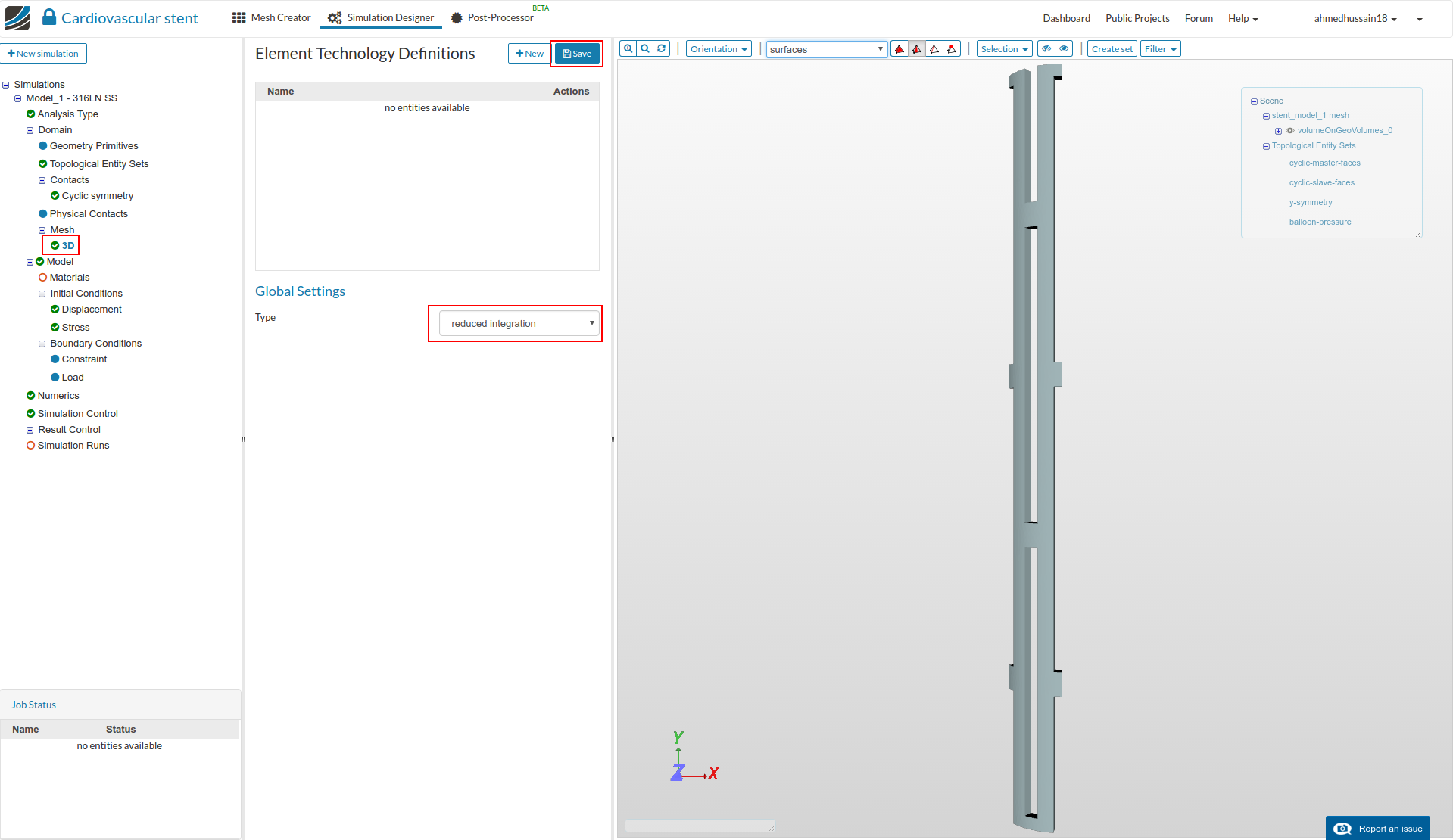
When dealing with a plastic material using second order elements, it’s always recommended to use reduced integration element technology to get more realistic results.
In order to do so, go to the 3D item in the Navigator under Mesh. Change the Type from standard to reduced integration.
Click Save to register the changes.
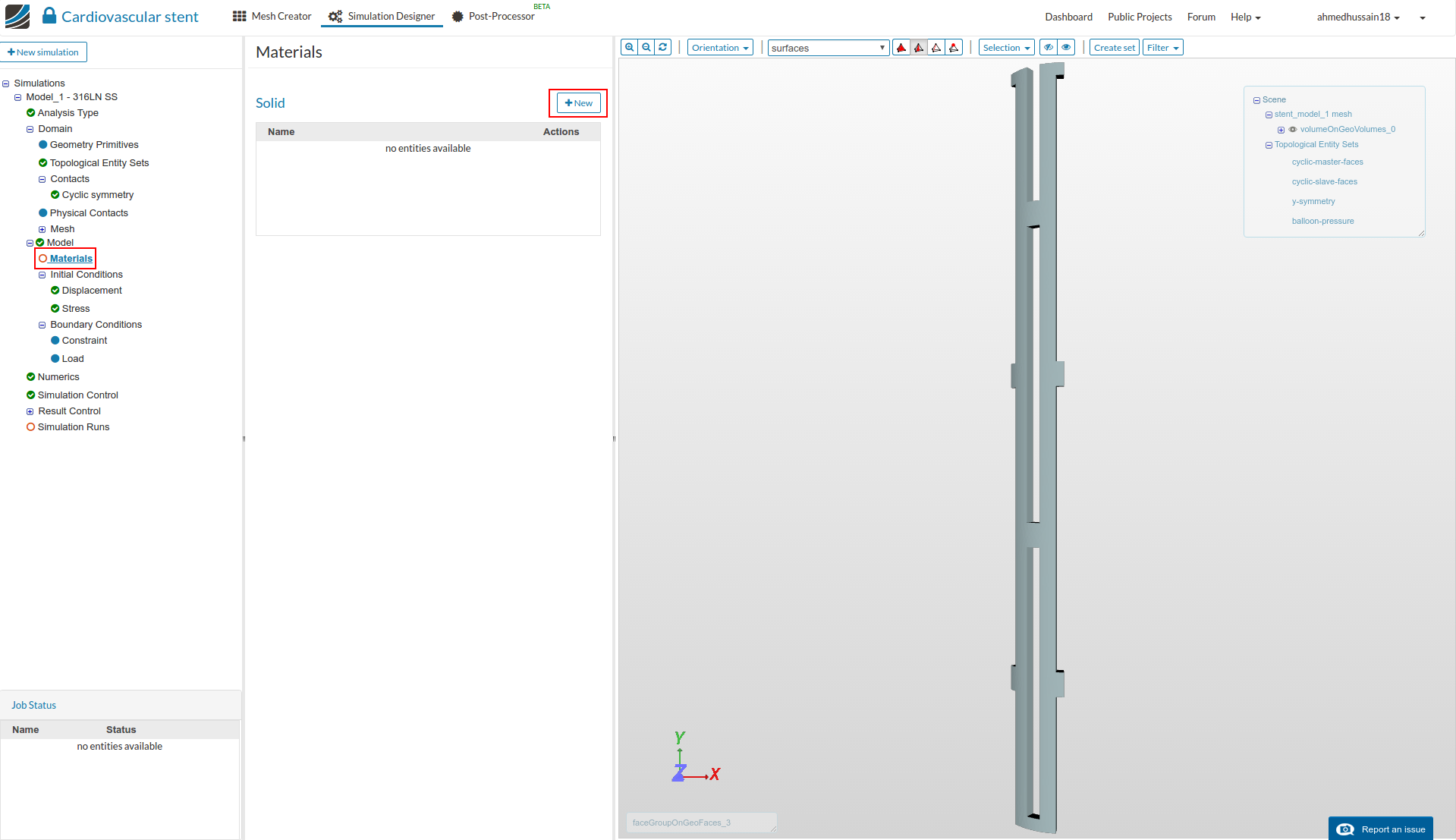
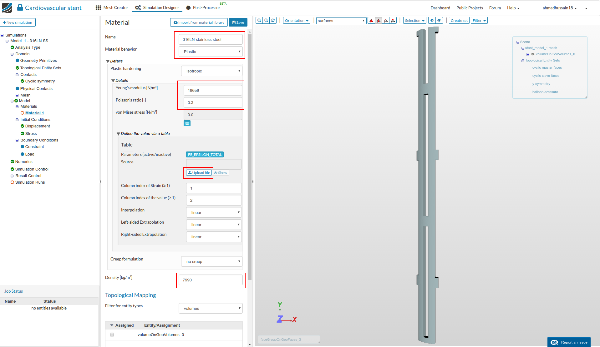
Now we will define the material definition for the stent. The material behavior is plastic since in reality the plasticity of the material is what allows the stent to remain in an expanded shape.
Go to the Materials item in the Navigator and click New to create a new material definition.
Rename the newly created material to 316LN stainless steel (optional). Change the Material behavior to Plastic.
Next, change the Young’s modulus, Poisson’s ratio and Density values to 196e9, 0.3 and 8800 as shown in the figure below.
Now we will create a .csv file with our plastic material data.
The stress strain data in this .csv file will start from yield point of 316LN steel. Just copy the values given below into Notepad (if you don’t have Notepad, you can download it for free here).
In Notepad, save the file as a .csv file e.g. stress_strain_316LN.csv (material data is taken from [1])
>     strain,stress
>     0.001046,2.0500E+08
>     0.005978,2.1140E+08
>     0.014505,2.2709E+08
>     0.026718,2.4502E+08
>     0.040775,2.6372E+08
>     0.059093,2.9062E+08
>     0.073767,3.0932E+08
>     0.089669,3.2877E+08
>     0.108644,3.4973E+08
>     0.129474,3.6995E+08
>     0.153392,3.8945E+08
>     0.174238,4.0744E+08
>     0.195088,4.2469E+08
>     0.218444,4.3600E+08
>     0.240578,4.4581E+08
>     0.264566,4.5489E+08
>     0.284253,4.6171E+08
>     0.307629,4.7004E+08
>     0.335337,4.7617E+08
>     0.366124,4.8306E+08
>     0.387059,4.8765E+08
>     0.404294,4.9222E+08
>     0.423379,4.9681E+08
>     0.442465,5.0139E+08
>     0.464027,5.0450E+08
>     0.484982,5.0612E+08
>     0.504087,5.0773E+08
>     0.526280,5.0861E+08
>     0.549081,5.1098E+08
>     0.570036,5.1260E+08
>     0.600000,5.1500E+08
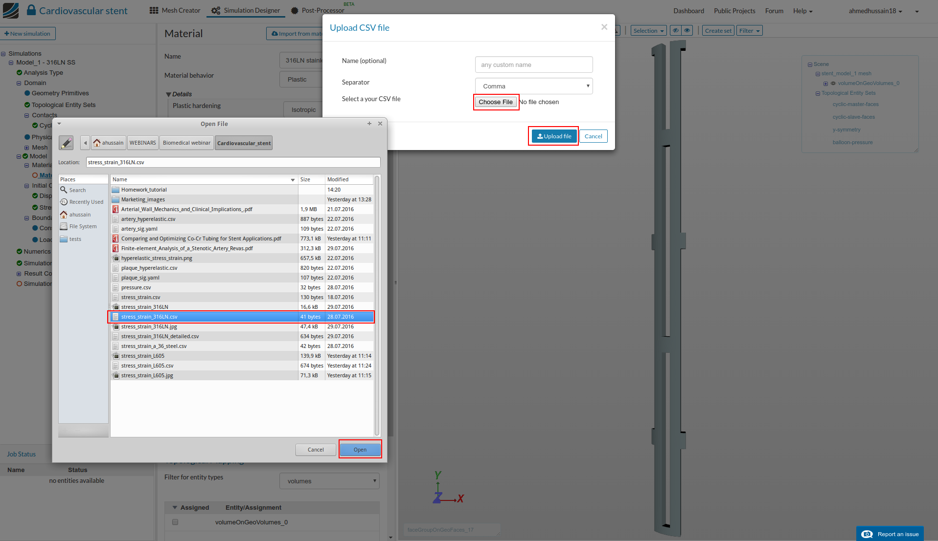
After creating the file upload it to SimScale by clicking Upload file in the Material Parameters. A pop-up window will open, click Choose file and open your created file from your computer and then click Upload file as shown in the figure below.
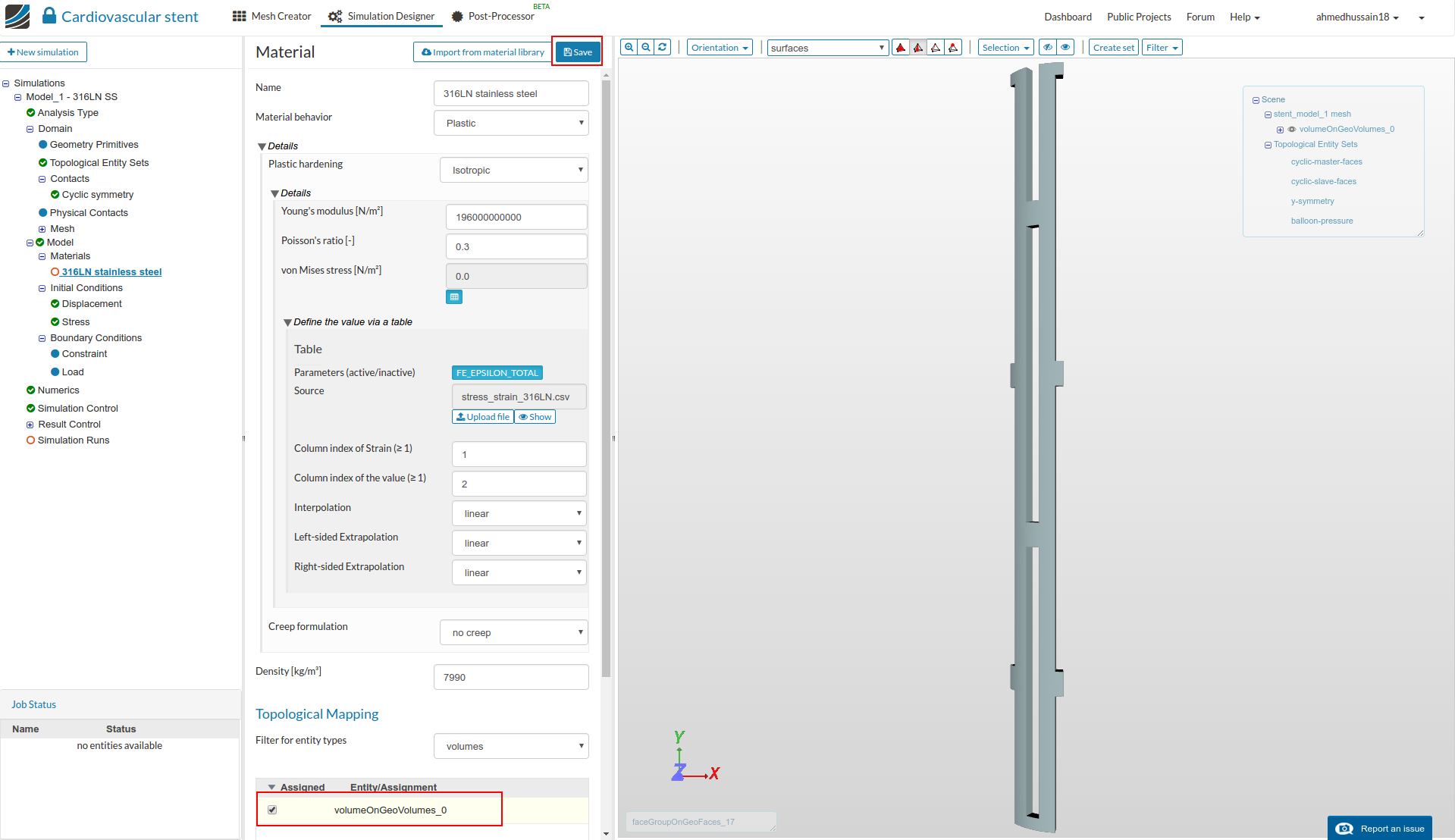
Finally, select the volume under Topological Mapping and click Save to define the material for this stent.
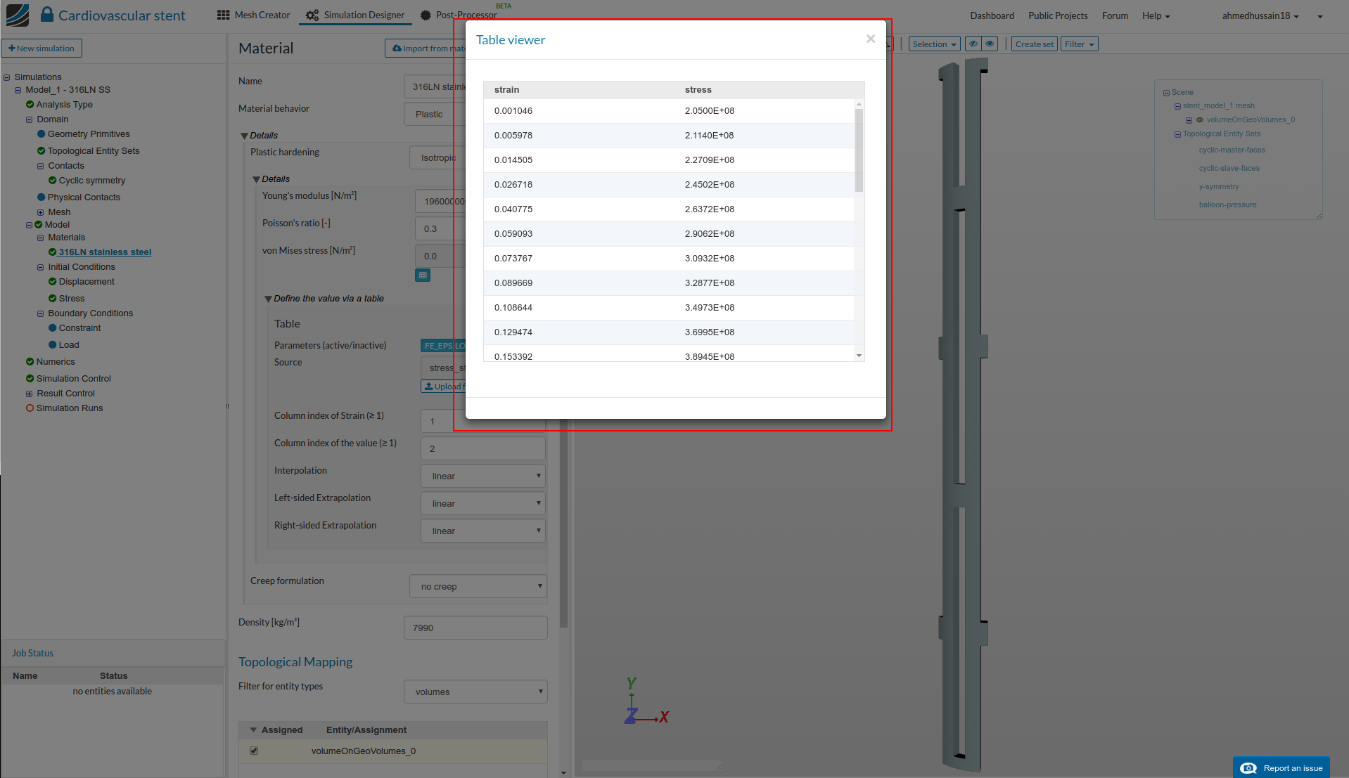
You can click Show to see the material data which should look something like this:
For more information on how to define plastic material, please see this forum post: Defining elastoplastic material
Now we will proceed with the constraint and load definitions for our simulation
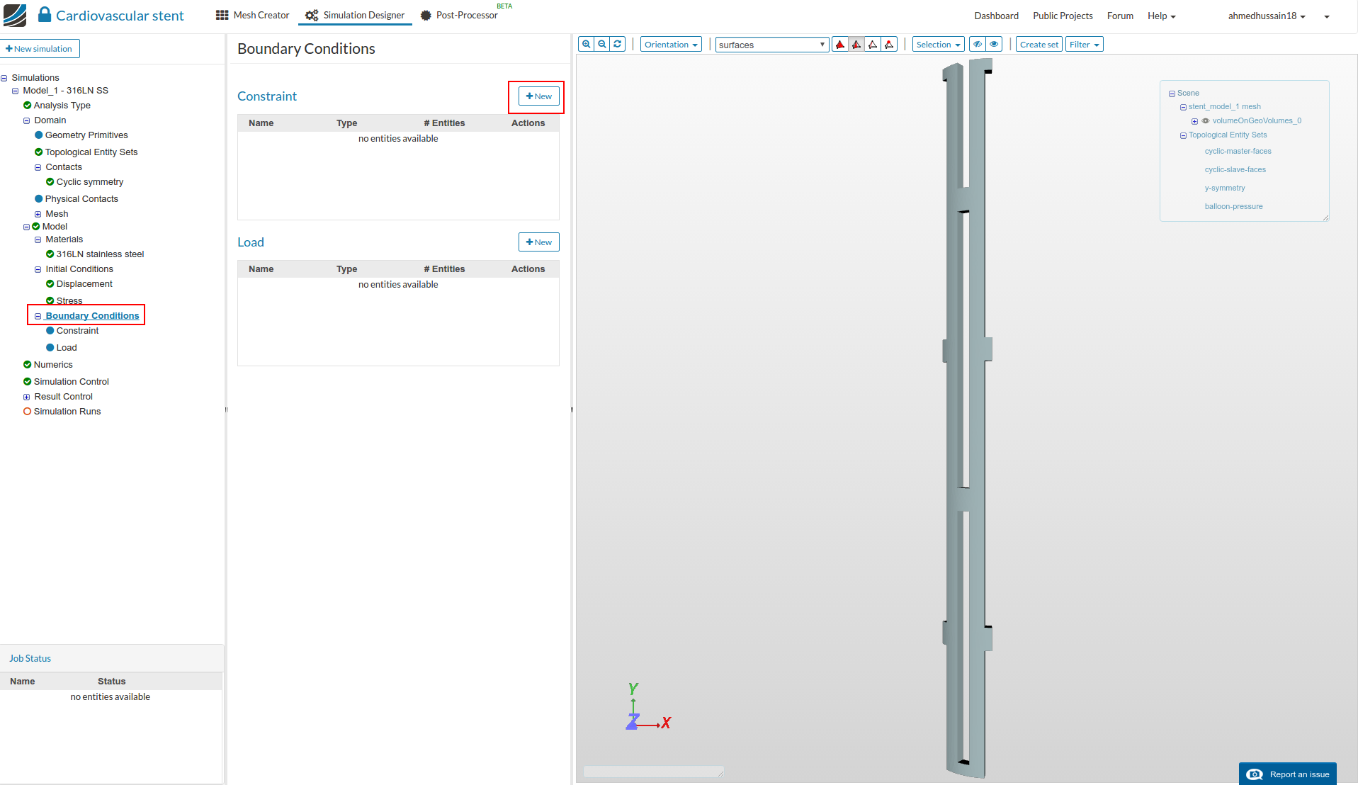
Go to the Boundary Conditions item in the Navigator and click +New next to Constraint to define the symmetry boundary conditions.
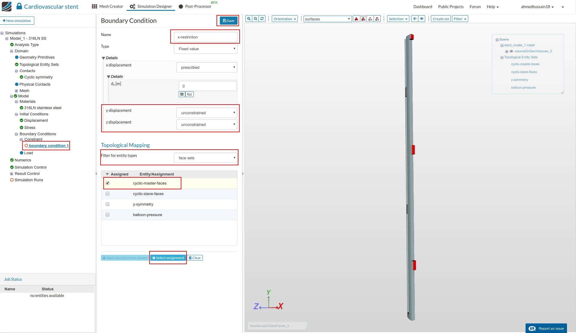
x-restriction:
We now have to define the restriction of the x-axis so that the geometry cannot move in the x-direction. Rename the newly created boundary condition to x-restriction (optional). Set y displacement and z displacement to unconstrained.
Change the Filter for entity types to face sets under Topological Mapping and select cyclic-master-faces
Click Select assignment to highlight the selected assignment in viewer. Click Save to save the constraint.
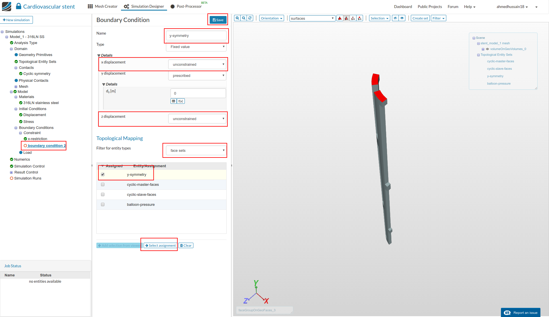
y-symmetry:
We now have to define the symmetry along the xz-plane so that the geometry shouldn’t be allowed to move along the y-axis thus maintaining the symmetry along the xz-plane. Do the same process as before and rename the newly created boundary condition to y-symmetry (optional). This time set x displacement and z displacement to unconstrained.
Change Filter for entity types to Face sets under Topological Mapping and select y-symmetry, click Select assignment to see highlight the selected assignment in the viewer. Click Save to save the constraint.
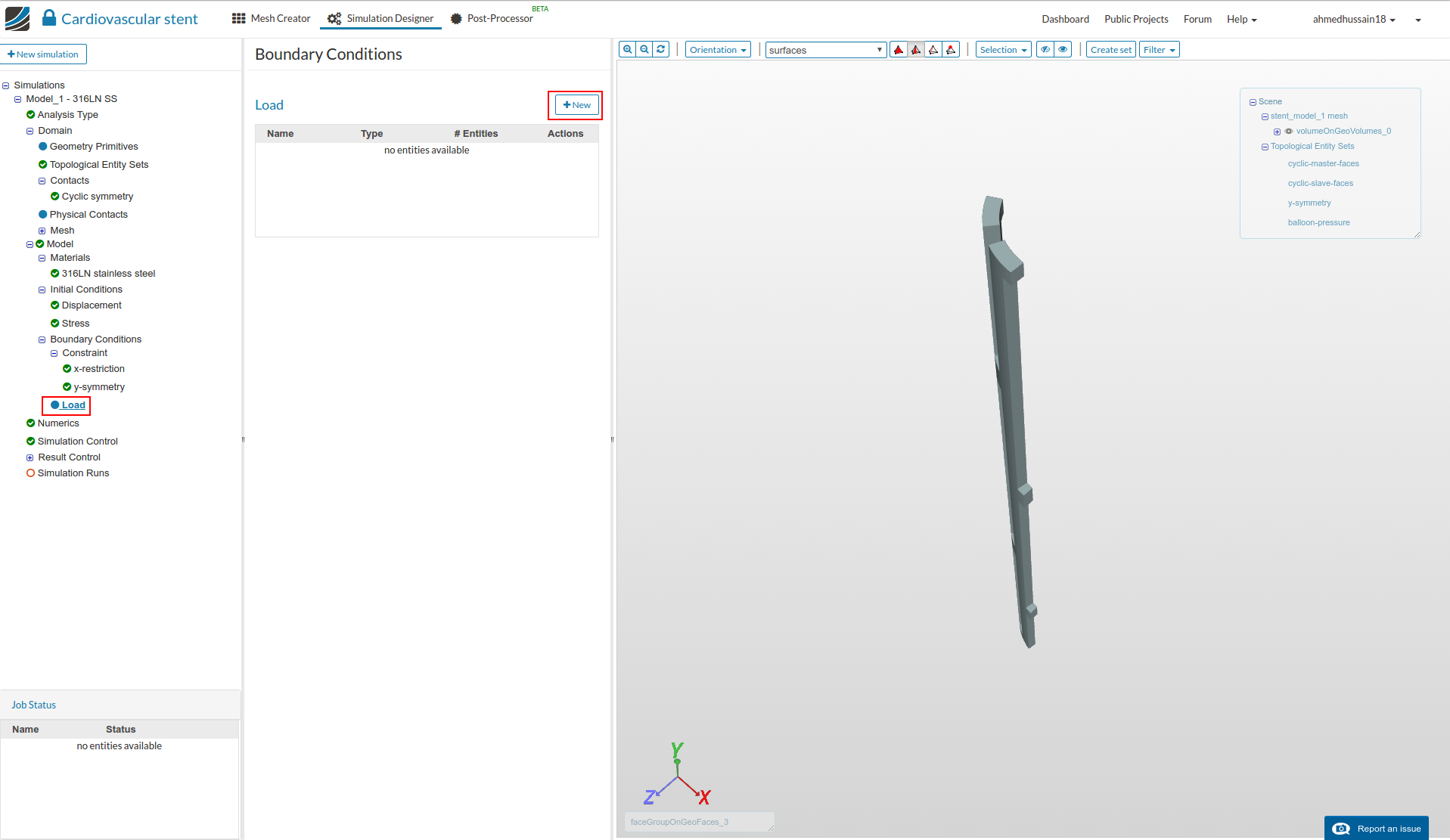
Load:
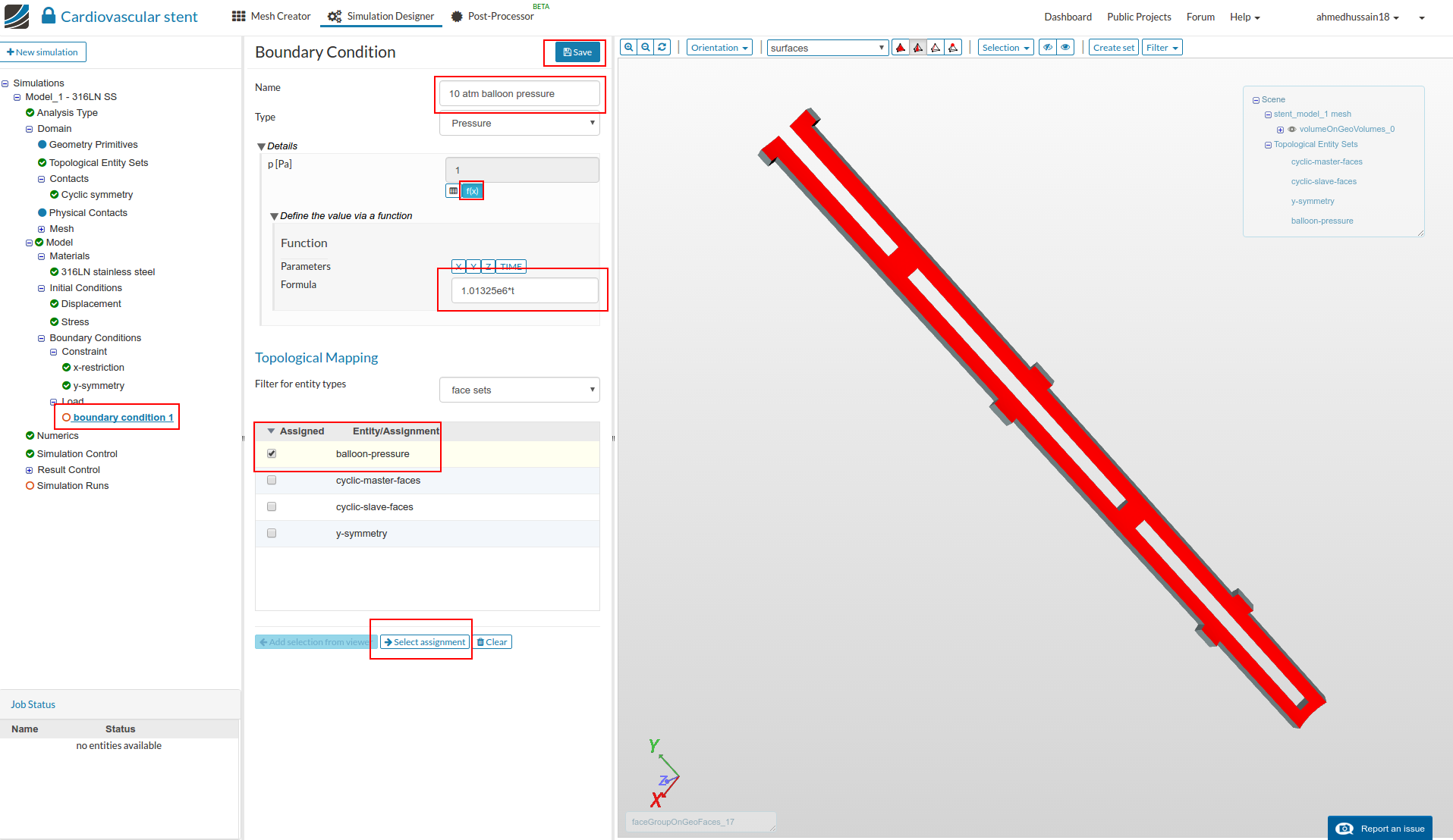
Next we will define our load boundary condition of the balloon pressure on the internal surface of the stent. Proceed to the Loads item in the Navigator and click +New to create a new load definition.
Rename the newly created constraint to 10 atm balloon pressure (optional). Click the f(x) button below the pressure value and input 1.01325e6*t, this will ramp the load over time since this is a nonlinear case
Go under Topological Mapping and select balloon-pressure, click Select assignment to see the selected assignment highlighted in the viewer. Click Save to save the constraint.
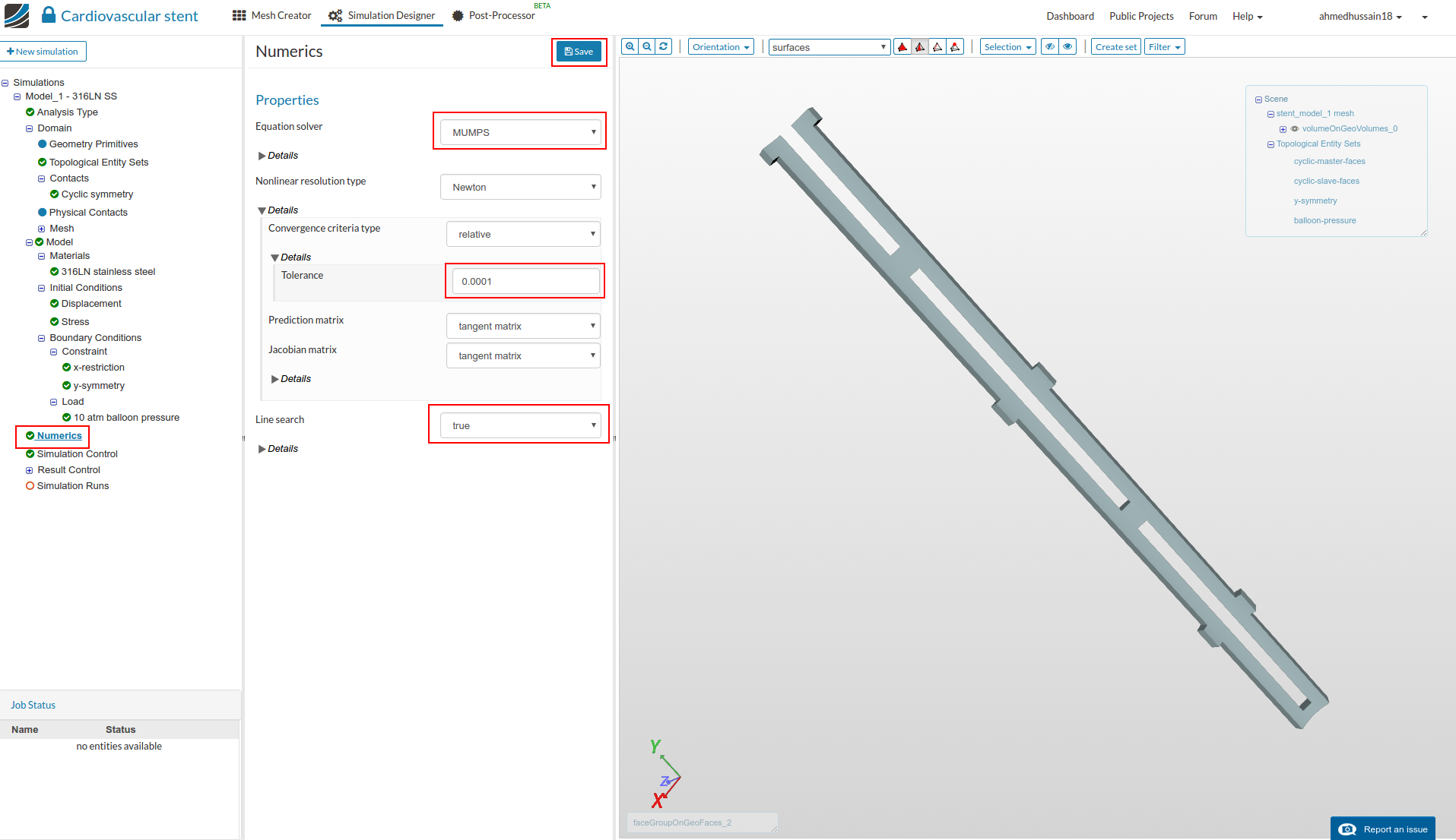
Go to the Numerics item in the Navigator and change the Equation Solver to MUMPS which is a faster solver for large nonlinear problems. Next change the Tolerance of relative error to 0.0001 under Convergence criteria.
Turn Line search to true which allows better convergence in case of material nonlinearity.
Click Save to register these changes.
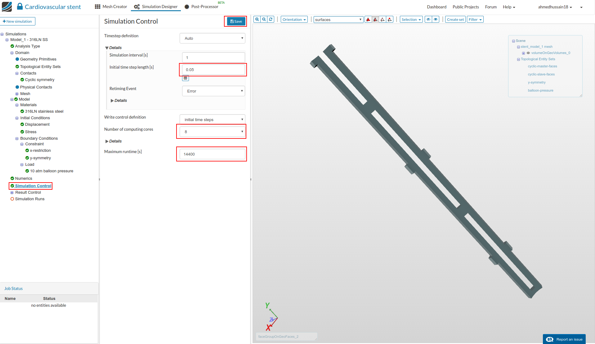
Click on Simulation control and change the Initial time step length [s] to 0.05, Number of computing cores to 8 and Maximum runtime [s] to 14400.
Click Save to register the changes.
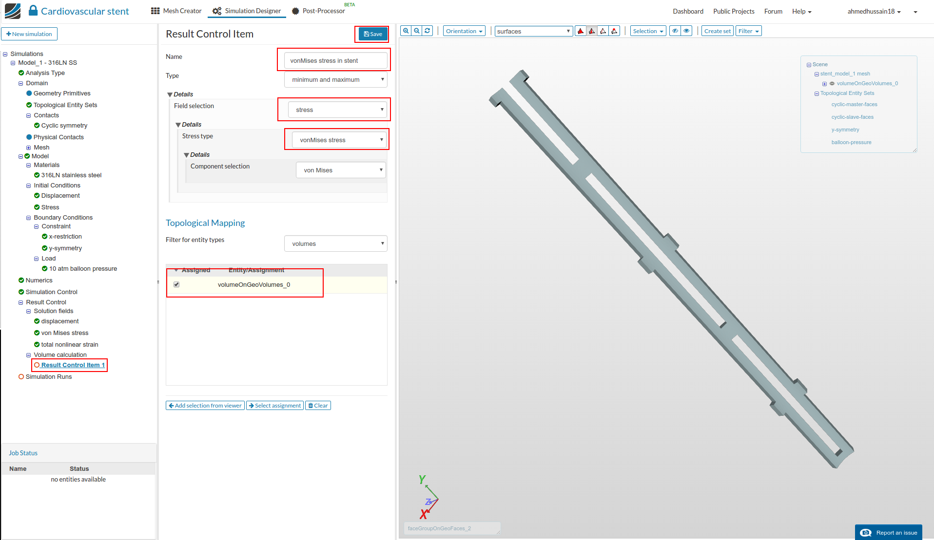
Next we will delete the cauchy stress solution field in order to save time and memory. Do this by right clicking on it and then selecting delete. The Solution fields will then look like as shown in figure below. Next click +New next to Volume calculation to create a new volume calculation definition.
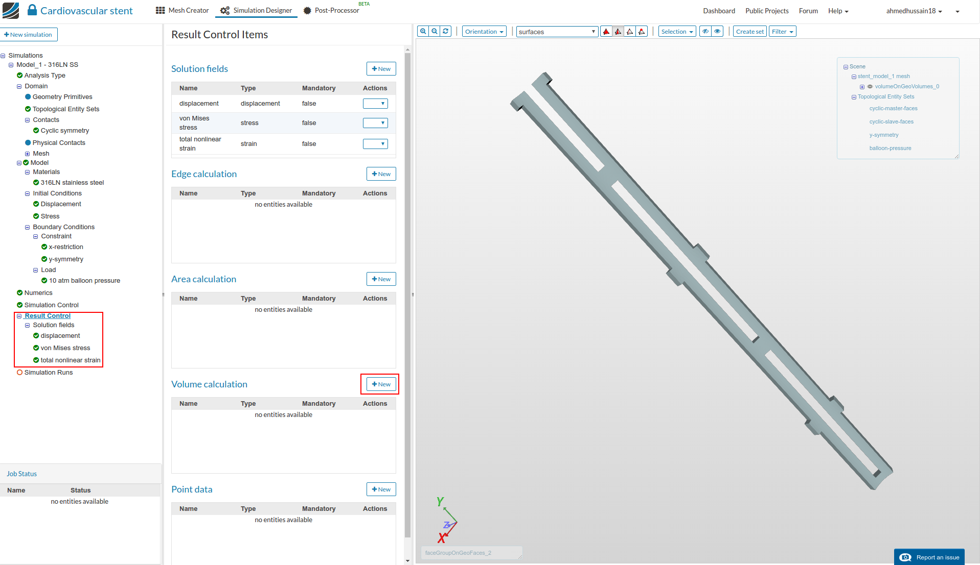
This will create a new volume calculation definition which will help us to plot the maximum and minimum von Mises stress in the stent over time. Rename it to von Mises stress in stent (optional), change Field selection to stress, Stress type to vonMises stress and then select volume from the Topological Mapping.
Click Save to define the volume calculation method.
Now we are ready to create our first simulation run. Click on Simulation runs and create a New run. Give simulation run a suitable name in the pop-up window that appears e.g. Run - model 1 - 316LN (optional) in this case.
Click Create to create a new run.

The new run will be created under Simulation Runs. Click Start to run the simulation.
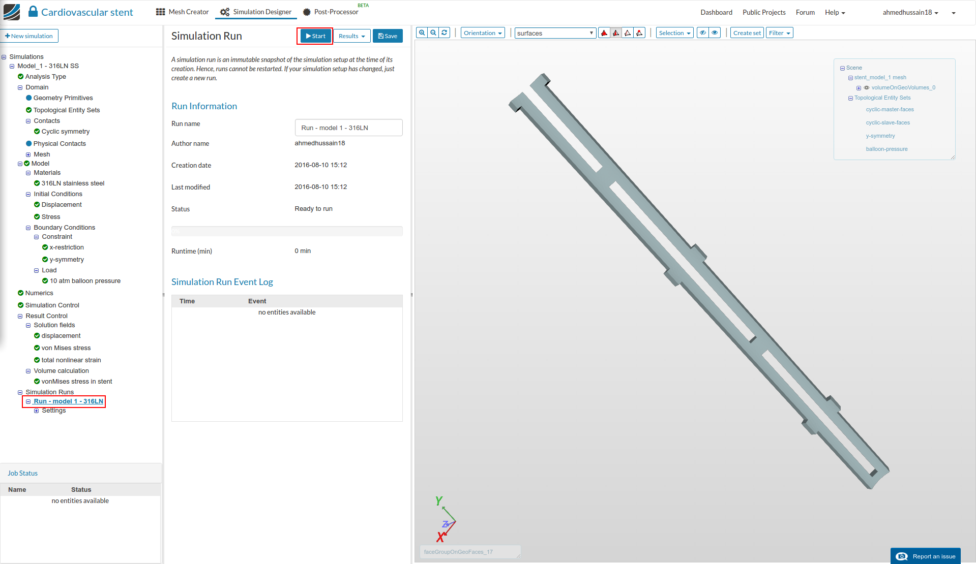
The simulation run will take approx. 35 minutes to finish. Now you can proceed to configurations 2 , configuration 3, and configuration 4
Configuration 2:
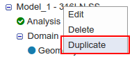
Once you have started the run with the first configuration setup, go ahead and make a duplicate of this simulation in order to perform the simulation with different material type for hip joint (configuration 2).
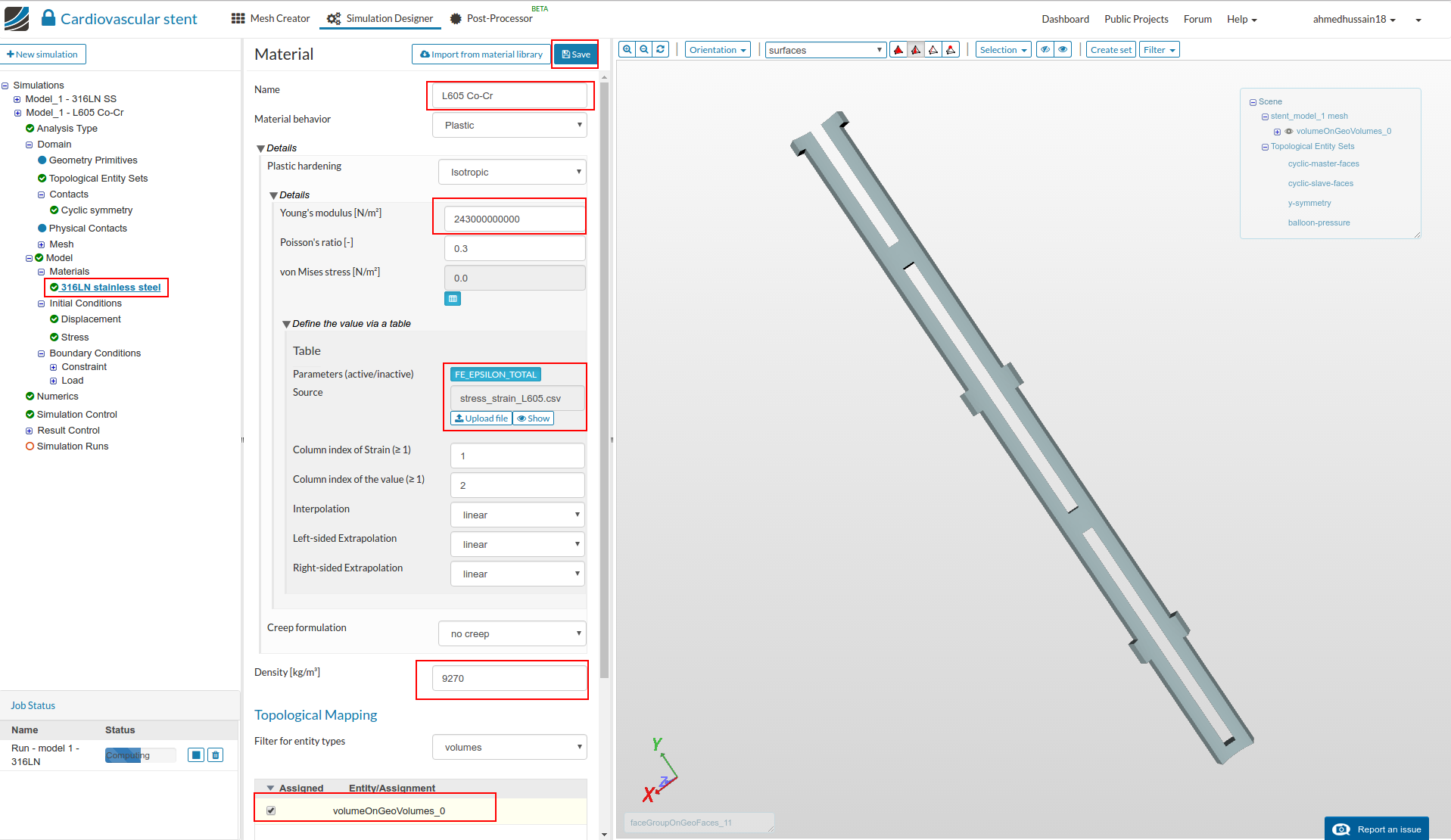
Rename the simulation to Model_1 - L605 Co-Cr and click Save
You need to first change the material definition of stent to L605 Co-Cr. Click on ‘316LN stainless steel’ under Materials, rename it to L605 Co-Cr (optional). Change the Young’s modulus, Poisson’s ratio and Density values to 243e9, 0.3, and 9270 as shown in figure below.
Now create the new .csv file by following the same steps as before with the stress strain data given below (material data is taken from [2]):
>     strain,stress
>     2.0580E-03,5.0000E+08
>     6.3241E-03,5.3200E+08
>     1.4625E-02,5.8250E+08
>     2.4111E-02,6.3250E+08
>     3.3202E-02,6.7000E+08
>     4.2688E-02,7.1000E+08
>     5.2174E-02,7.5000E+08
>     6.4427E-02,7.9250E+08
>     7.5889E-02,8.2250E+08
>     8.9328E-02,8.5500E+08
>     1.0119E-01,8.7750E+08
>     1.1621E-01,8.9750E+08
>     1.3004E-01,9.1250E+08
>     1.4348E-01,9.2500E+08
>     1.5771E-01,9.3000E+08
>     1.7510E-01,9.4250E+08
>     1.8854E-01,9.4750E+08
>     2.0395E-01,9.5250E+08
>     2.1976E-01,9.5750E+08
>     2.3597E-01,9.6000E+08
>     2.5534E-01,9.6500E+08
>     2.7510E-01,9.7500E+08
>     2.9723E-01,9.8250E+08
>     3.1976E-01,9.9500E+08
>     3.4625E-01,1.0050E+09
>     3.7233E-01,1.0125E+09
>     4.0040E-01,1.0225E+09
>     4.1937E-01,1.0325E+09
>     4.3715E-01,1.0400E+09
>     4.5652E-01,1.0475E+09
Click Save to save the new material definition.
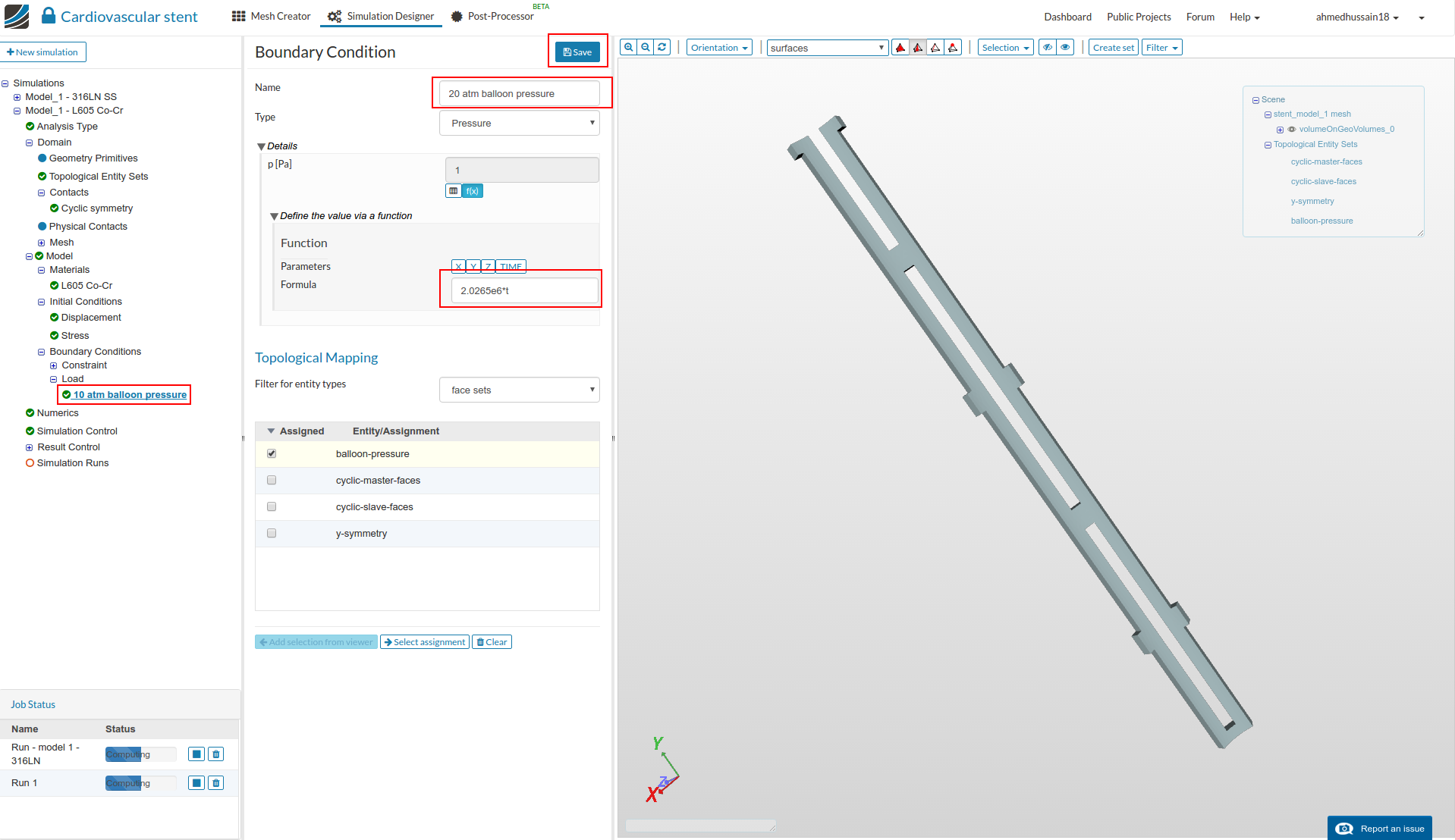
Next change the 10 atm balloon pressure to 2.0265e6*t and rename it to 20 atm balloon pressure (optional).
Click Save to register changes.
Create a new run and rename it to Run - model_1 - L605 Co-Cr (optional) and then click Start.
Configuration 3:
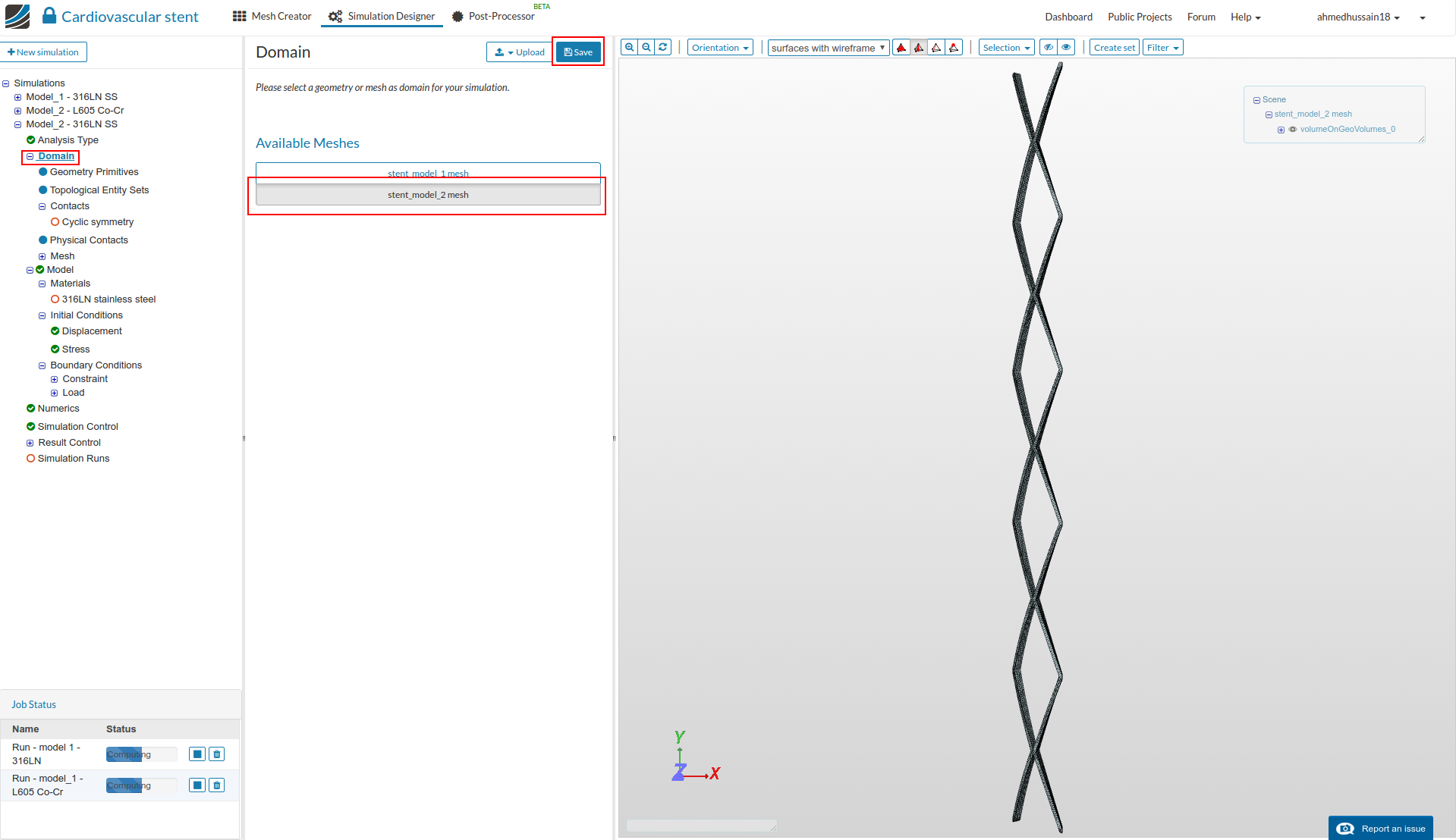
For the 3rd configuration, duplicate the simulation Model_1 - 316LN SS simulation, rename it to Model_2 - 316LN SS and click Save.
Now you have to change the Domain to stent_model_2 mesh and click Save. Click Yes on the warning message. Soon the viewer will be updated with the second mesh.
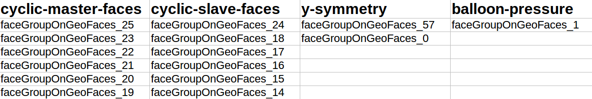
Now create the topological entity sets. In this case the sets will have following number of faces.
The table below shows the faces selected for each topological entity set:
After creating the sets, you have to reassign the entities for the Materials and Boundary conditions. Also you have to reassign the volume to Volume calculation under Result Control.
Finally create a new run and rename it to Run - model 2 - 316LN (optional) and click Start.
Configuration 4:
For the 4th configuration, duplicate the simulation Model_1 - L605 Co-Cr simulation, rename it to Model_2 - L605 Co-Cr and click Save.
Now you have to change the Domain to stent_model_2 mesh and click Save. Click Yes on the warning message. Soon the viewer will be updated with the second mesh.
Now create the topological entity sets. In this case the sets will have following number of faces.
The table below shows the faces selected for each topological entity set:
After creating the sets, you have to reassign the entities for the Materials and Boundary conditions. Also you have to reassign the volume to Volume calculation under Result Control.
Finally create a new run and rename it to Run - model 2 - L605 Co-Cr (optional) and click Start.
Post-processing
Once the simulation is over, click on Post-processor tab to view the results.
Select Solution fields of the simulation run you want to view results. In this case it is Run-case 1 - 316LN.
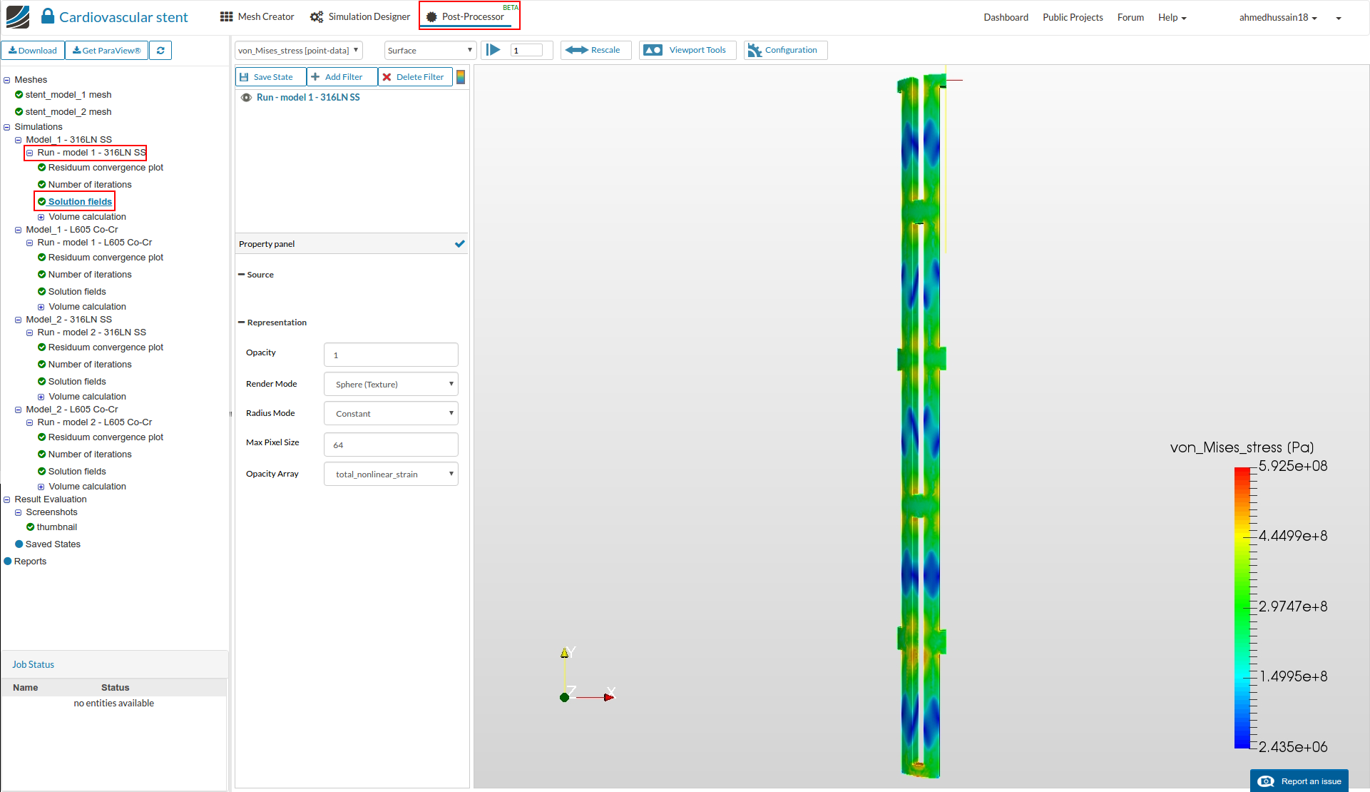
In order to view the deformed shape, click on Add Filter and then Warp by Vector. You will see a Warp by Vector filter is added under your solution field and in the result viewer, the deformed bone will appear with the undeformed shape.
You can select Toggle color bar to view the magnitude of the von Mises stress (right side of the Delete Filter button).
Hide the undeformed shape by clicking on eye icon to the left side of Run - Case 1 - 316LN.

-
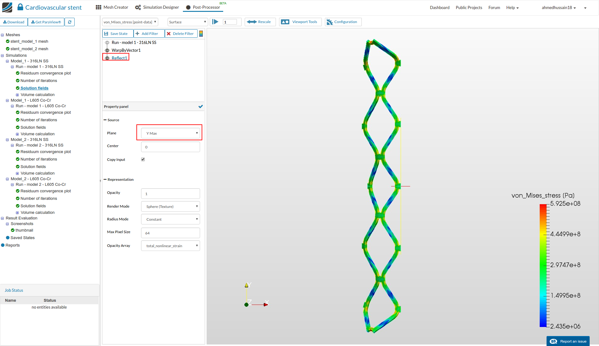
This result is only a section of the complete geometry. In order to see the whole deformed geometry, we need to reflect this result along positive y-axis and transform it along circumferential direction.
-
First we will reflect it along positive y direction. Click on Add Filter and then Reflect.
-
Choose Y Max for Plane and click on Apply to apply the changes. You will see that the deformed geometry is reflected about the plane normal to the Y-axis.
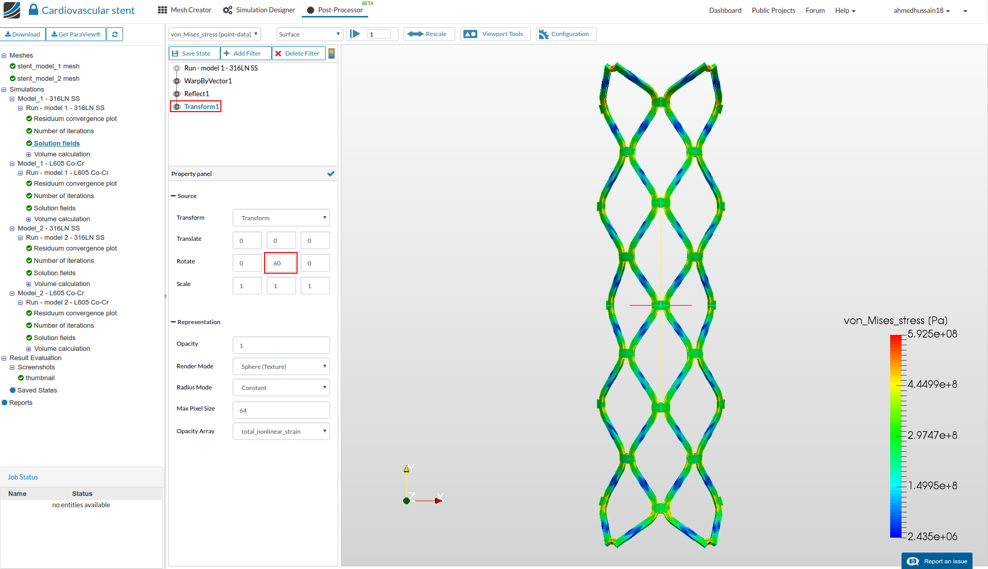
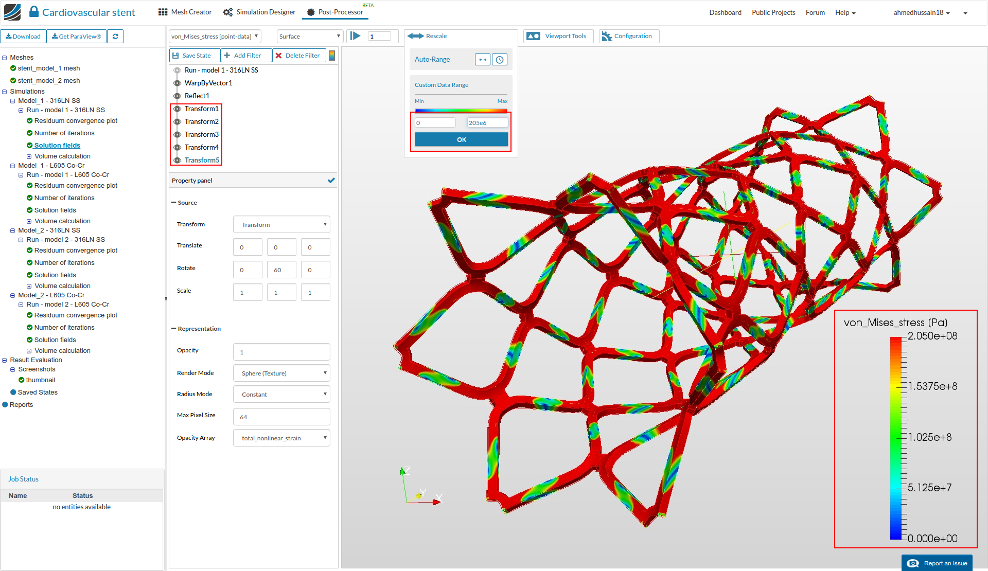
Now we will copy this result along the circumferential direction. For that, we use the Transform filter and specify 60 in the second column of Rotate since our axis is along the Y axis.
-
Repeat this step 5 times to get the get the complete deformed geometry.
-
Rescale the vonMises stress values from 0 to 205e6 and click OK to see which portions of the stent have yielded.
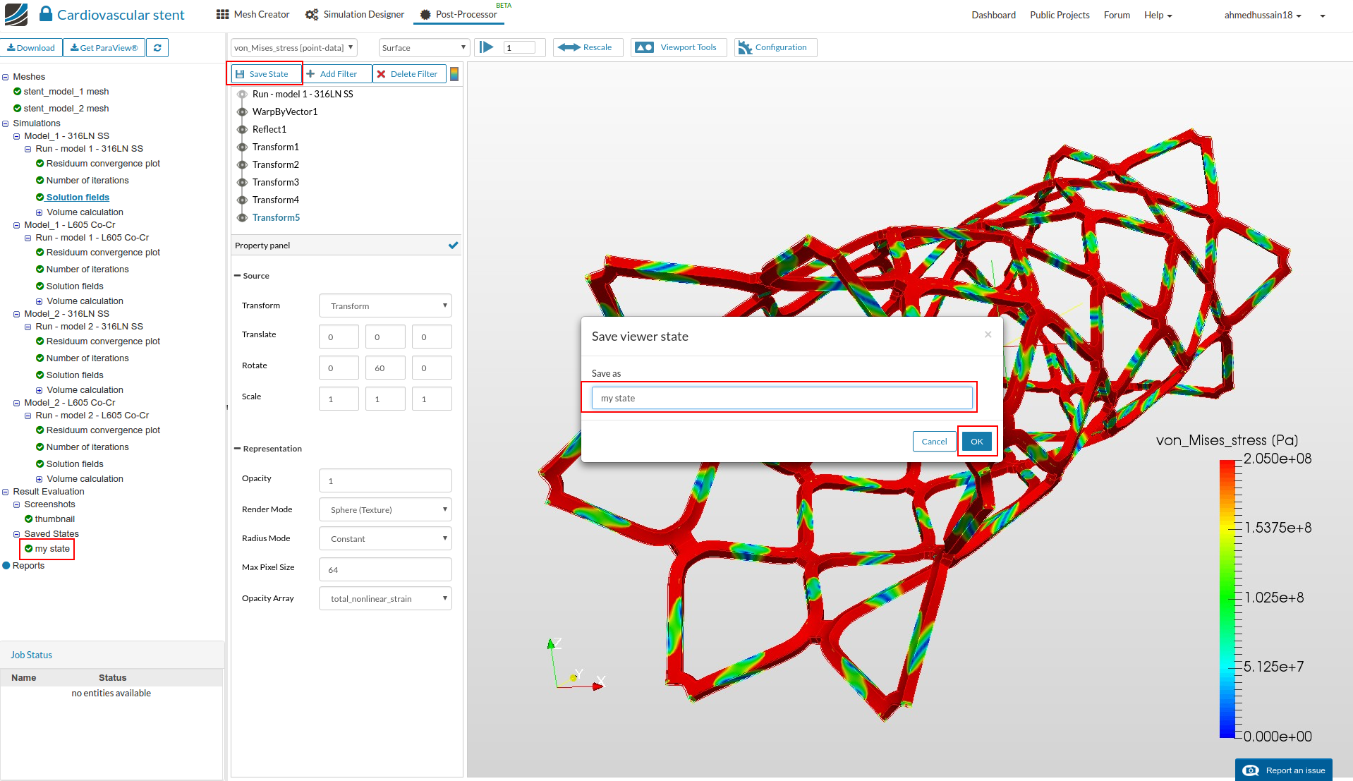
- You can save the state in order to use it later. Click Save State, give a reasonable name and click OK to save the state. The saved state will appear under the saved state tree menu on the left.
- In order to see the animation, click the play button which will animate all the saved 20 steps.
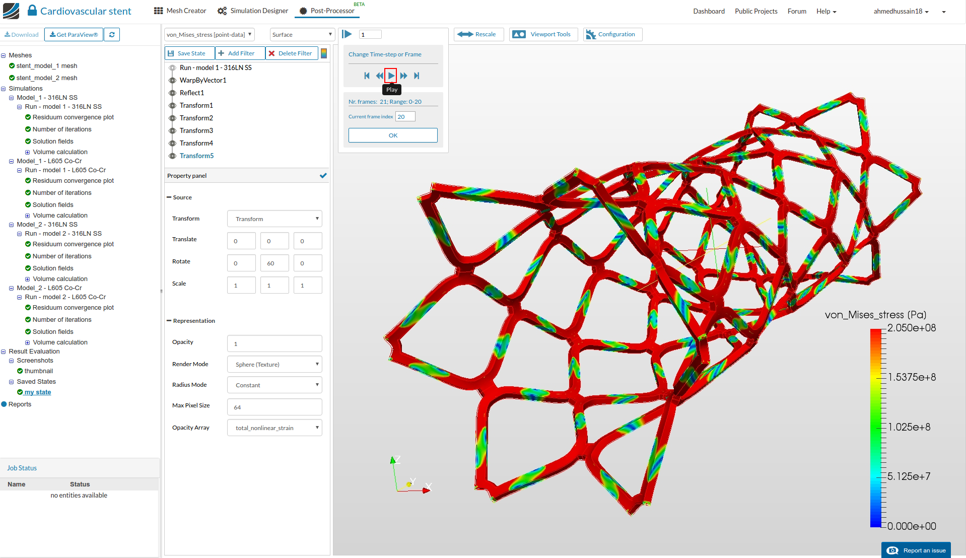
- The animation will look something like this:
-
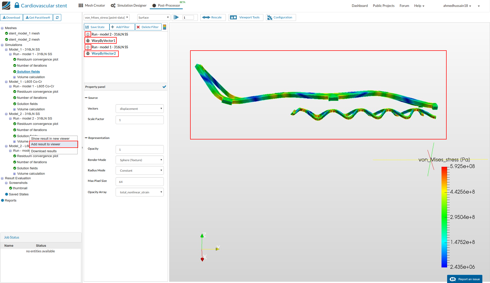
To compare other configuration’s results, we will load the solution by right clicking on the respective Solution fields and then Add to result viewer.
-
Apply the WarpByVector filter on both cases and hide the actual solution fields by clicking the eye icon next to them.
-
You will then see the deformed shape of both cases. It is worth noting that the stent model 2 is expanded considerably less compared to the first model case, but the second model expansion is more uniform than the first one.
References:
[1] AURICCHIO∗, Ferdinando, M. Di Loreto, and E. Sacco. “Finite-element analysis of a stenotic artery revascularization through a stent insertion.” Computer Methods in Biomechanics and Biomedical Engineering 4.3 (2001): 249-263.
[2] Poncin, P., et al. “Comparing and optimizing Co-Cr tubing for stent applications.” Proceedings of the materials and processes for medical devices conference. 2004.