AIJ Case E: Building complexes with simple building shape in an actual urban area (Niigata)
Overview
The purpose of this project is to use experimental results from the Architectural Institute of Japan [1] to validate CFD results gained from SimScale. The case being validated is Case E, which consists a complex of buildings with simplified geometry. Many scenarios are presented in Case E, The scenarios used to validate the SimScale platform were the North, East, South and Westerly winds for the after construction scenario.
The SimScale CFD results were compared to the experimental results and found to have good correlation. Some underprediction was seen in the k-epsilon models in the strong wind regions and underprediction in the wake regions, but is a known trait of the K-epsilon model and is acceptable and should be considered when evaluating results.
Geometry
The geometry was converted into STL using Bear File Converter [2] and imported into SpaceClaim to turn the mesh into solids. The solids were then subtracted from a larger volume which was to be the surrounding fluid domain. To do this a certain amount of cleaning had to be done, including creating thin cylinders on edges which touched but wasn’t intersected. This was the cause of some CAD issues external to SimScale.
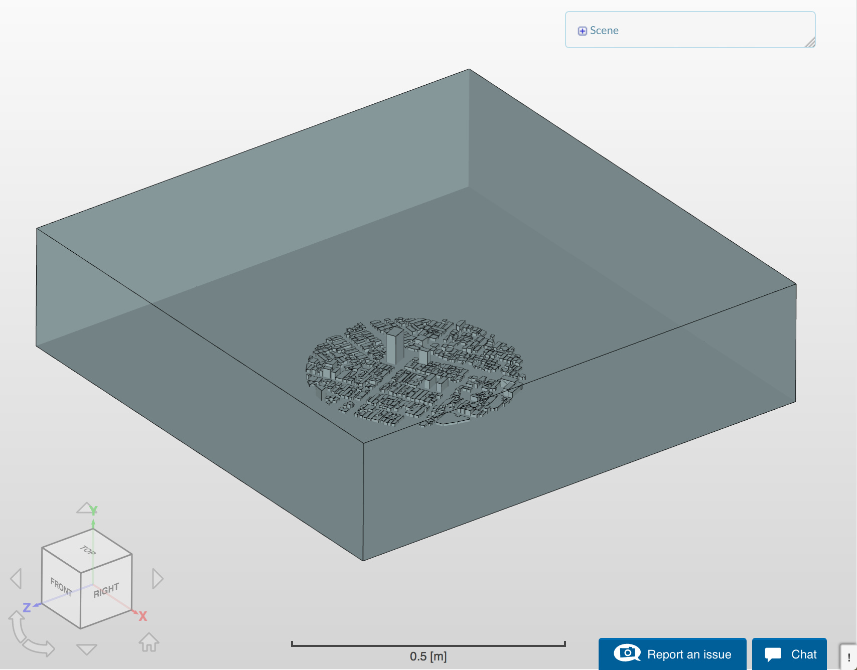
Figure 1: Domain and city geometry used.
The geometry was then imported to SimScale as a STEP as the geometry was simple and doesn’t require splitting to be able to assign individual walls that were required in the result controls later. The bounding box was two kilometres by two kilometres and a single kilometre high.
Mesh
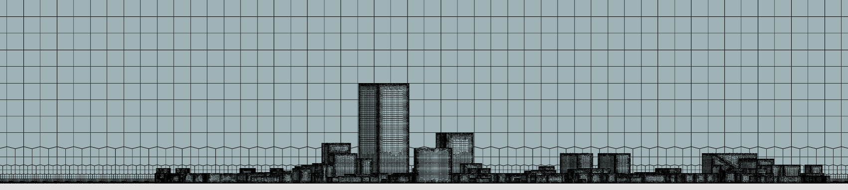
The mesh used was a parametric hex-dominant mesh, where region refinements were placed on the city itself and further surface refinements on the building faces. The floor was refined with a thin region refinement. The floor and the buildings had two layers inflated relative to the cell size.
Figure 2: Mesh refinement around city (top) and looking across the city (bottom)
The above images show that the vase mesh was quite coarse, with a cell density of 50/km. A feature refinement was used to ensure edge quality was preserved to a refinement level of 6, whilst the building surfaces were refined to a level maximum level of 5 and a minimum of 3 to ensure that the mesh didn’t join when there were thin channels between buildings. The outer city refinement was to a level of 2 whereas the inner city refinement which was upon the lower city only was to a level of 4. The cell count for the mesh was 30 million cells.
Model
The model type was steady state with the k-epsilon turbulence model. The standard air material was used and the solution was initialised using potential flow.
These validation simulations were all set up similarly, with only the inlet, outlet and side faces being altered depending on wind direction. The inlet was defined using a CSV upload for velocity, turbulent kinetic energy and dissipation rate and a zero gradient pressure condition. The outlet was a zero pressure outlet and the top and sides were slip walls. The buildings and the ground were no-slip condition walls.
The gradient schemes were altered from default to be cell limited gauss linear schemes, and the solution used 2 non-orthogonal correctors and the relaxation factors were found to be most efficient at a uniform 0.3. The simulations were run to a tight convergence in 6000 iterations, where all residuals fell below 1e-5 except pressure which fell below 1e-4. Average values were monitored for velocity convergence on the domain walls (except the bottom) and a force result control was placed on the large centre building to ensure that the solution was steady in the region where most measurements were taken.
Results
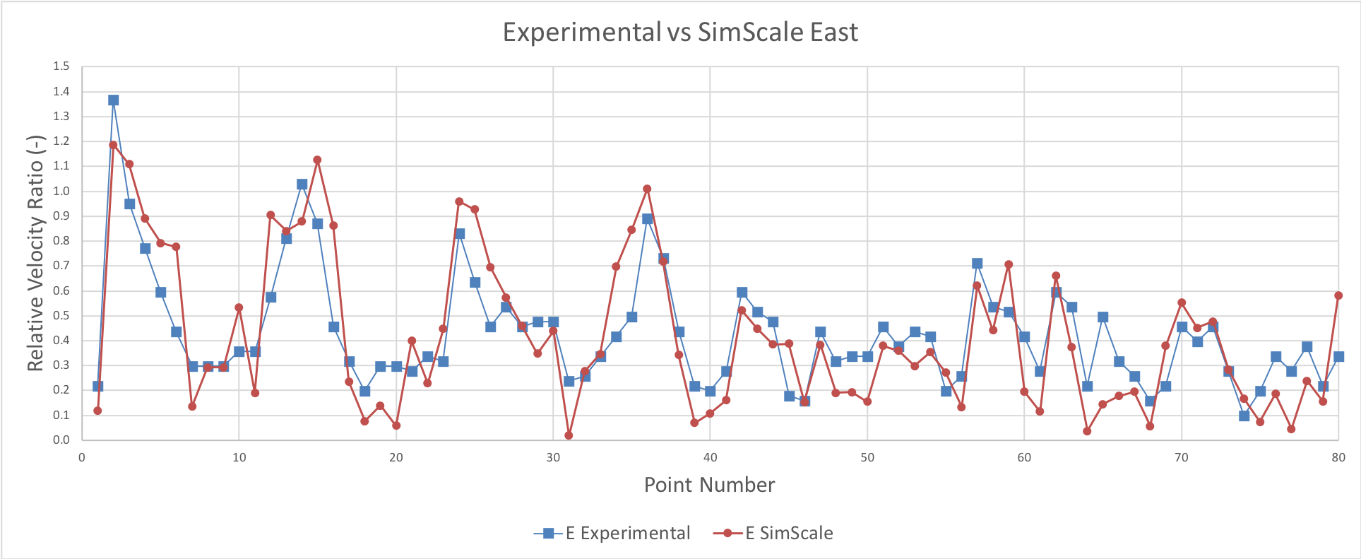
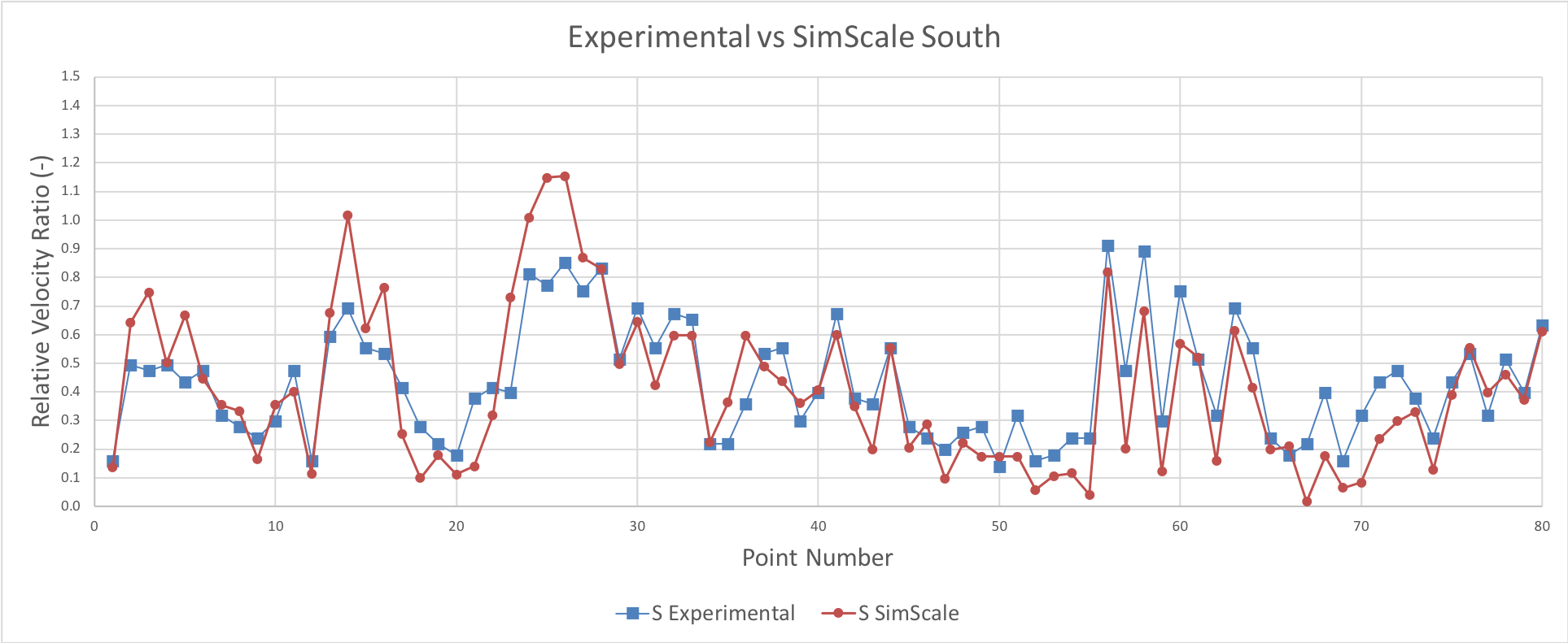
To compare the results to the experimental results provided, the velocities were normalised with the value of velocity at the inlet at a height of 15.9m. The measurements were taken at points listed in [Source].
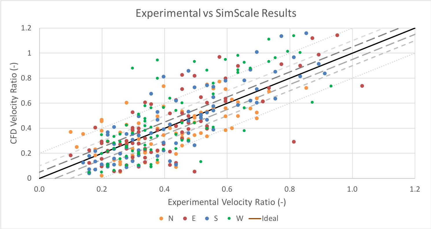
To compare the results as a whole, the CFD results obtained from the SimScale platform were plotted against the experimental results to see the correlation for cases North, East, South and west after construction.
Figure 3: Correlation between experimental and SimScale CFD results for cases North, East, South and Westerly winds after construction.
The correlation between experimental and SimScale results was highly linear, with a majority of the points being within 0.2 in relative velocity. To see how the results compared in more detail the results were plotted against the point numbers so they could be compared to the velocity slices.
Figure 4: Points positioning in relation to strong Northerly winds and building wakes.
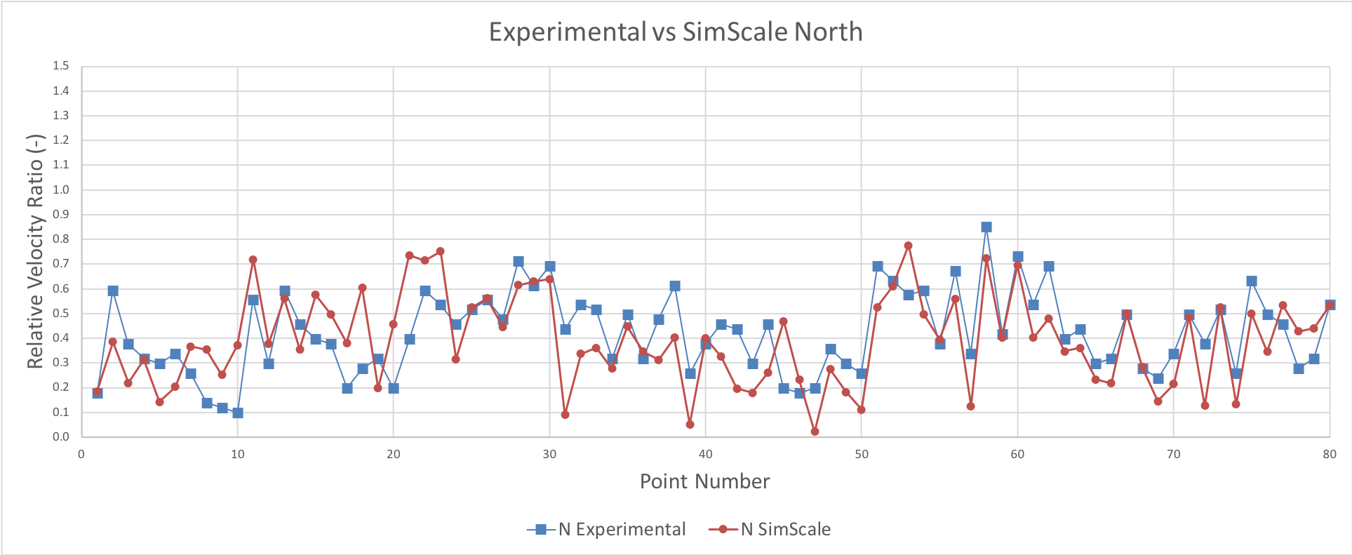
Figure 5: Relative velocity comparison between Experimental and SimScale CFD results for a northerly wind.
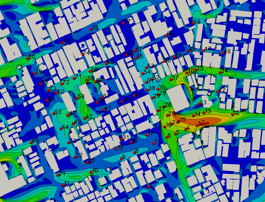
Figure 6: Points positioning in relation to strong Easterly winds and building wakes.
Figure 7: Relative velocity comparison between Experimental and SimScale CFD results for a Easterly wind.
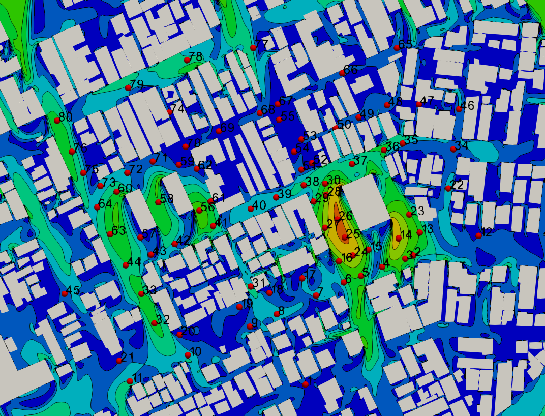
Figure 8: Points positioning in relation to strong Southerly winds and building wakes.
Figure 9: Relative velocity comparison between Experimental and SimScale CFD results for a Southerly wind.
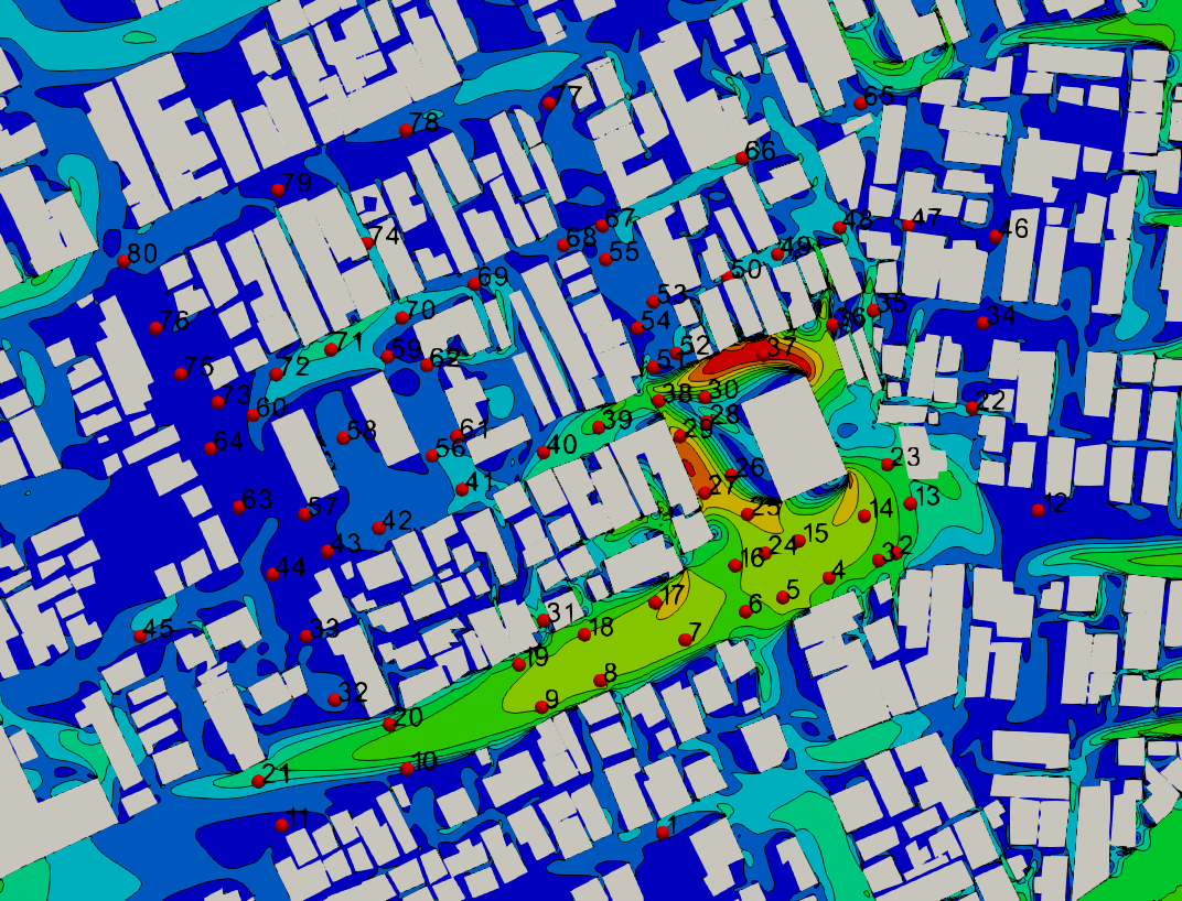
Figure 10: Points positioning in relation to strong Westerly winds and building wakes.
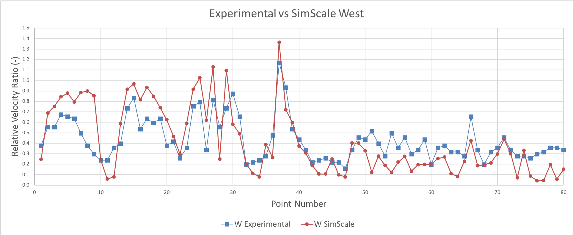
Figure 11: Relative velocity comparison between Experimental and SimScale CFD results for a Westerly wind.
The results above show that as the correlation plot suggested the simulated result bare very similar results. It can be observed that in regions of particularly high velocity, the simulated results slightly over predict in comparison to the experimental results. This might be considered more desirable than under prediction as this is where wind comfort is likely to be an issue. In contrast, points located in wake regions tend to be under predicted, this is not normally considered an issue since the places where wind comfort is an issue isn’t usually in the wake regions. Examples of this are most strongly seen in the westerly wind scenario. This is a known trait of the K-epsilon model.
References
[1] AIJ, Guidebook for Practical Applications of CFD to Pedestrian Wind Environment around Buildings. Guidebook for CFD Predictions of Urban Wind Environment
[2] Bear File Converter, DXF to STL conversion. DXF to STL | Bear File Converter - Online & Free