AIJ Case D: High-rise Building in City Blocks
Overview
The purpose of this project is to use experimental results from the Architectural Institute of Japan [1] to validate CFD results gained from SimScale. The case being validated is Case D, which consists of a single high-rise building, surrounded by blocks of simplified buildings. The geometry used was the scaled geometry from the data file provided by the Architectural Institute of Japan [3], and measurements were taken at points also listed in the data file.
Mesh
The scaled model was surrounded by a 1.8m x 1.8m x 1.8m bounding box, with 25 cells in each direction. The buildings surfaces and edges were refined to maintain geometrical accuracy, and the lower region between buildings was refined to ensure a sufficient amount of cells were present between the buildings.
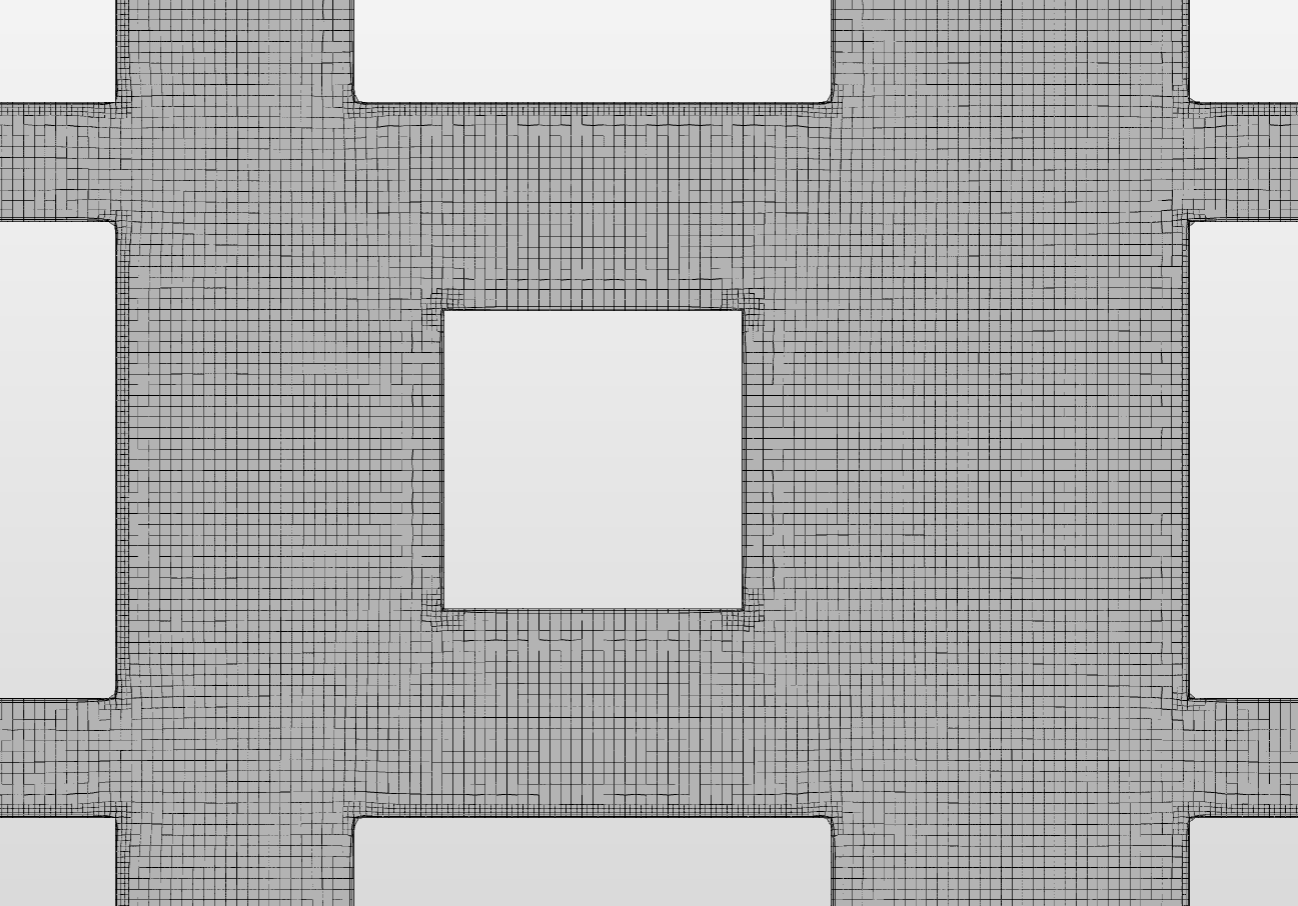
Figure 1: Mesh size, showing wireframe of bounding box cells.
Figure 2: Mesh around the area of interest, sufficiently refined in thin channels and feature refined at the edges. Two layers are visible on the building surfaces.
Simulation Setup
For all cases an incompressible steady flow was used and when comparing to measurements from the Split Fiber Prob, at zero degrees flow angle (in the direction of the x-axis) both a K-Omega SST and K-Epsilon model were used. When comparing to the Thermintor Anemometer results, just the K-Epsilon model was used for 0, 22,5 and 45 Degrees. Wall modelling was employed on the ground and buildings, whereas a slip condition was used for the domain sides and top. A zero pressure outlet was used on the low X bounding box surface. In all cases a CSV upload was used for the inlet on the high X bounding box wall, defining velocity vectors, turbulent kinetic energy and either dissipation rate or specific dissipation rate, varying with height.
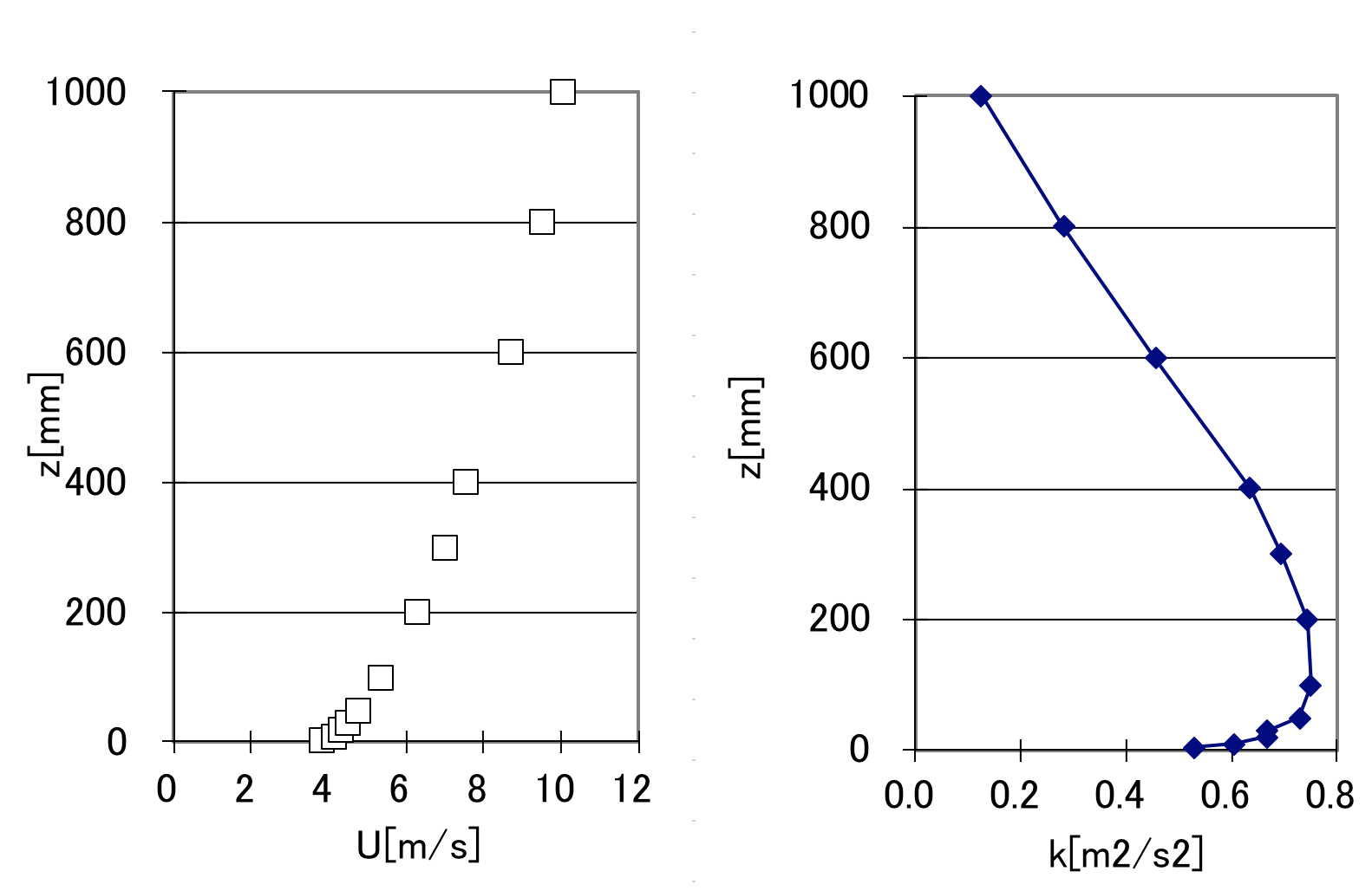
Figure 3: Velocity and Turbulent Kinetic Energy Profiles
A tight convergence was reached at around three thousand iterations in most cases, where residuals fell below 1e-5 for everything but pressure which settled at around 1e-3 to 1e-4. Velocity at the bounding walls were monitored for velocity convergence, and forces were measured on the high rise walls for pressure convergence around the area of interest. This also allows for the measurement of wind load on the the building.
Results
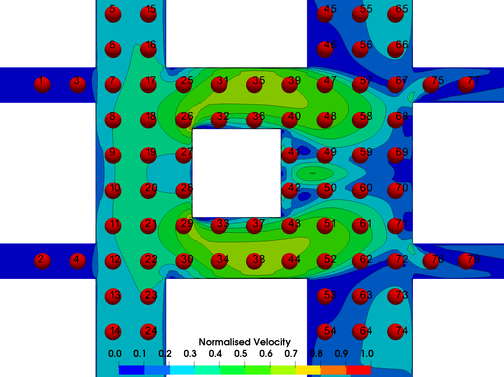
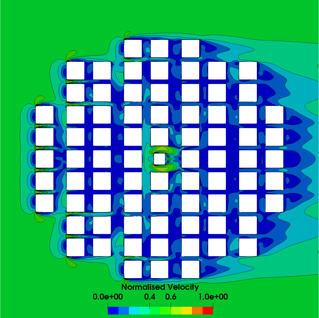
To compare the CFD results to the experimental results normalised velocity scalars were probed at locations defined in the data file for Case D [3]:
Figure 4: Slice showing Normalised Velocity field of the K-Epsilon results for 0 Degrees flow angle, points and text showing location and number of measured points.
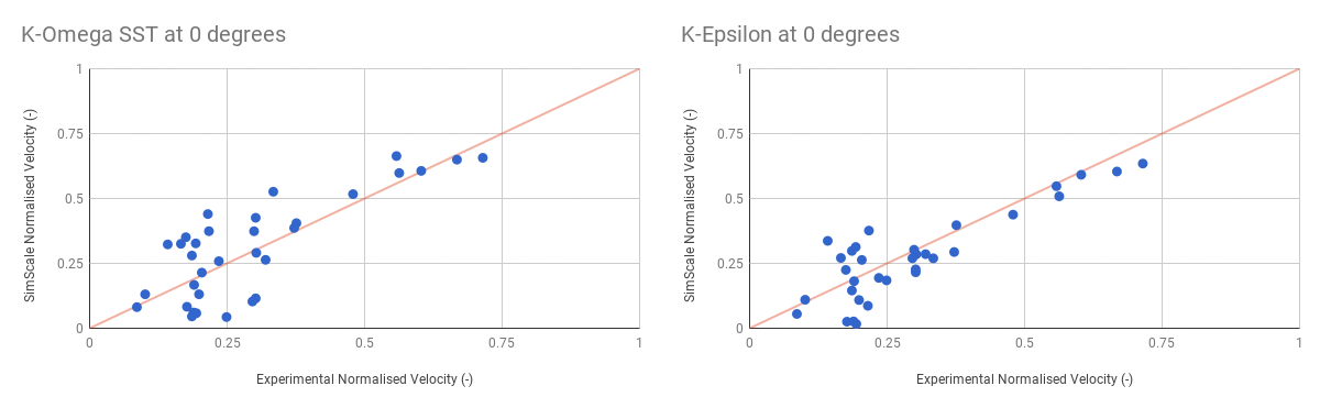
Plotting the CFD data against the Split Fiber Probe experimental data, it is desired to see a plot that is close to linear, if a perfectly linear set of results were observed it would represent identical results between, CFD and Experimental:
Figure 5: Showing K-Omega SST against Experimental (Left) and K-Epsilon against Experimental (Right).
The above plots show that both models produce very linear results with the K-Epsilon model showing a better linear correlation. The variance in results is expected and the measured points with high variance are likely to be located in wake regions.
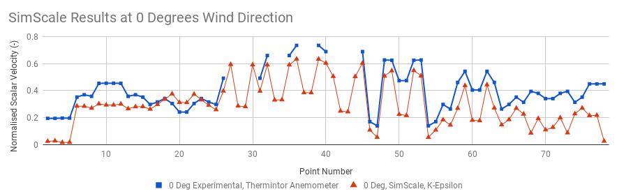
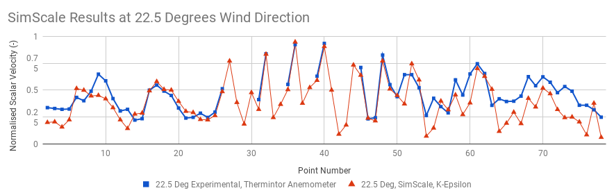
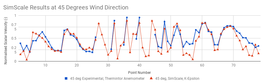
Plotting the results for the Thermintor Anemometer measurements against CFD results for flow angles of 0, 22.5 and 45 degrees will use a different type of plotting, for this we shall plot both as a series against point number to determine where variance occurs and trends in the data can be observed:
Figure 6: Experimental Data and CFD data from SimScale plotted at each point for 0 Degrees (Top), 22.5 Degrees (Middle) and 45 Degrees (Bottom).
These data sets show strong similarities between SimScale’s CFD data and Experimental results. Discrepancies can be seen in low velocity regions, where the CFD result report a lower velocity than the experimental results and as mentioned before is expected. It is noted in paper [2] that thermintor anemometer measurements will report slightly higher results due to the way the velocity magnitude is calculated, please refer to the paper for more details.
Figure 7: Normalised Velocity in the wider city, showing a planar slice at measuring height of 5mm.
The above plot shows the normalised velocity distribution on the plane of measurement, the region of interest around the center building shows that it has the highest velocity gradients on the plane where velocity speeds up around the building before rotating around into the buildings wake (Figure 8).
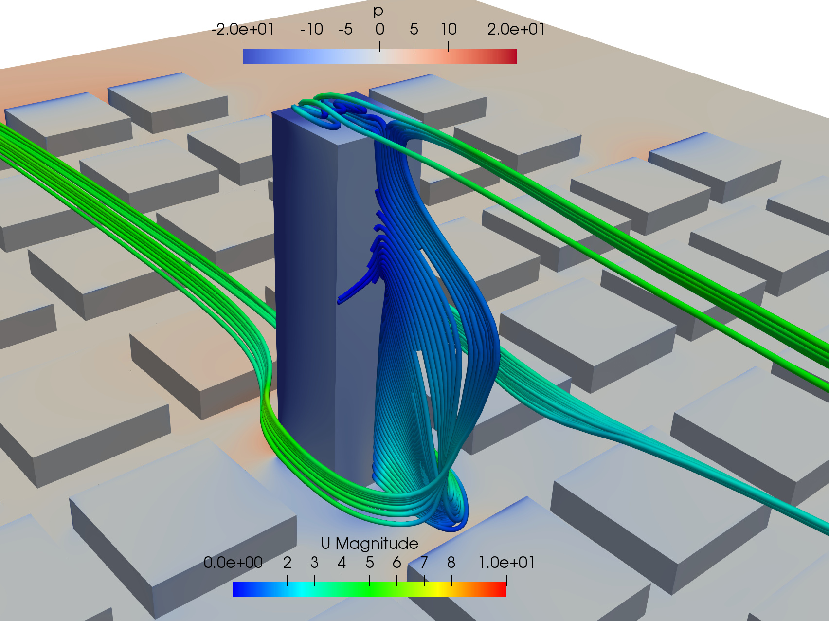
Figure 8: Pressure surface plots with stream tracers coloured by velocity magnitude.
References
[1] Guidebook for Practical Applications of CFD to Pedestrian Wind Environment around Buildings, Guidebook for CFD Predictions of Urban Wind Environment.
[2] Cross Comparisons of CFD Prediction for Wind Environment at Pedestrian Level around Buildings, 404 Not Found | 日本建築学会.
[3] Case D data file, https://www.aij.or.jp/jpn/publish/cfdguide/data/CaseD(Highrise+Blocks).xls.