A Short Discussion on Solvers

Hi all,

As much as it is going to sound like a feature request, it is not. I am bringing it up because I have followed SimScale for a while and haven’t noticed any trace that these following features are enabled. Your team may be already working on some of them.

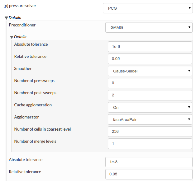
Firstly, I would like to ask what is the Krylov subspace method preconditioned by? From David’s recent reply to the GT350R simulation, it doesn’t look like it is preconditioned by multi-grid. There have been quite a few studies including my own testing that concluded multi-grid preconditioned (Bi) Conjugate gradient is faster than multi-grid by itself. While AMG results in a much faster convergence, Krylov subspace methods scale better in parallel computation.

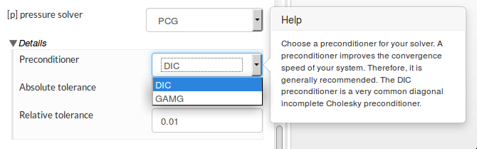
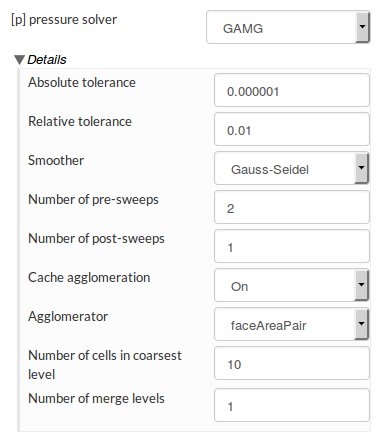
Secondly, I have noticed within AMG, one is not allowed to customise the solver. Things such as the number of pre/post sweeps and v-cycles ( 2 by default ), merge levels, smoother etc. In some case, speedup is significant by altering those parameters, specially when going with ILU a higher merge level can be used.

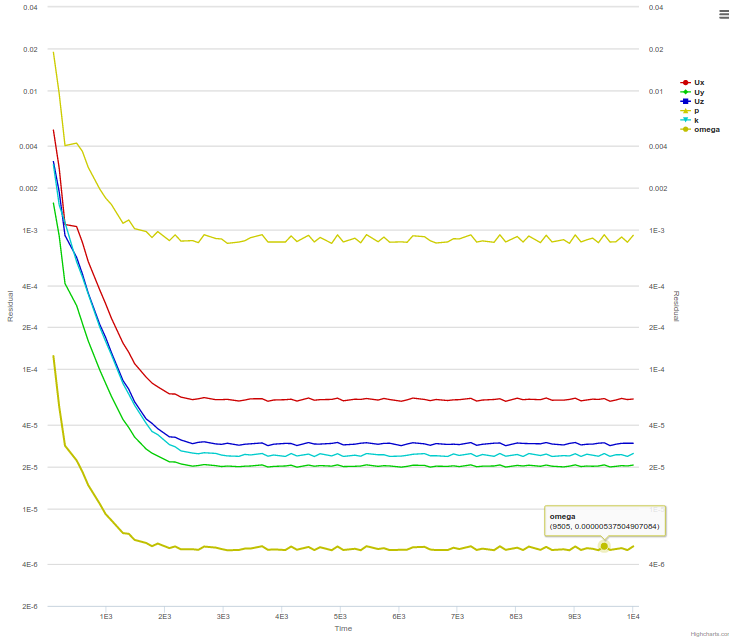
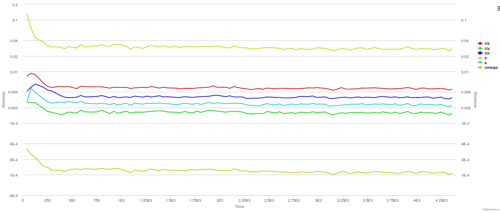
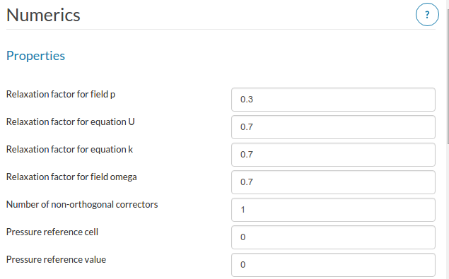
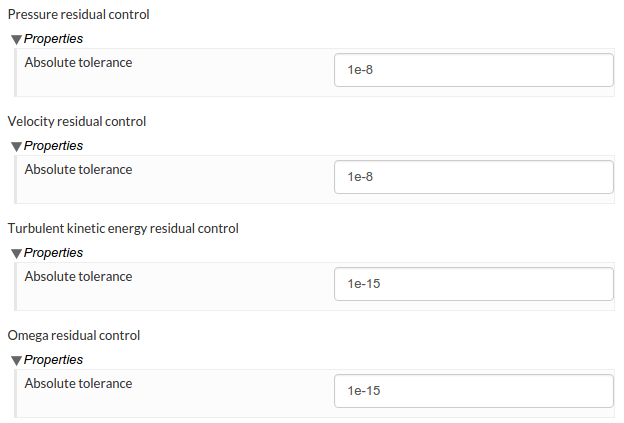
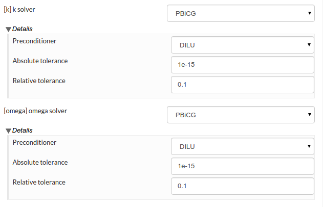
Thirdly, there doesn’t seem to be a relative tolerance control for steady state computation. It is very useful to use a large relative tolerance in steady state, because in this case it is the initial residuals at the start of each SIMPLE loop (time step) that matter, rather than the final residuals at the end of those loops. With a large relative tolerance, the solve will then quickly move onto a newer SIMPLE loop and therefore the initial residuals will drop more ( with more iterations ). The same outcome can be achieved by limiting max number of iterations within each loop.

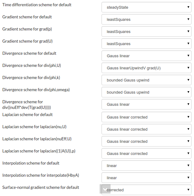
The second last point I would like to bring up is about the schemes available. Although there are a variety of discretisation schemes for convective terms, none of them seem adequate for scale-resolving computations. The limitedLinear is a central differencing with the Sweby limiter. This TVD scheme is less dissipative than linearUpwind but is, I believe, still far too dissipative for LES. The scheme I usually use for convective terms is LUST, while Gamma can be useful in a few cases. A pure central differencing can be too expensive to afford.

Finally, the SIMPLEC algorithm is significantly faster than SIMPLE when the flow field has a weak coupling in physics, as no pressure underrelaxation is required and larger underrelaxation factors can be used on the other fields ( velocities and turbulence parameters ). Examples of such flows are isothermal incompressible and mildly compressible flows. I have pretty much only used SIMPLC to compute external incompressible/compressible aerodynamics in steady state.

Looking forward to all of your replies.

1 Like

Nice question! Wish there would be more questions like yours in order to get a better understanding why you “click this and not another option” as it is often the case with programs.

@dylan, agree with @jousefm - interesting points you’re raising. A few thoughts/comments from me:

The symmetric system solvers currently offer an incomplete Cholesky and a multigrid preconditioner, see screenshot below:

The general idea behind the SimScale user interface is that the user can tweak the details of a simulation setup but he isn’t forced to do so. This is why a lot of settings, first look like this:

and if you expand them, they look like this:

So you do get access to most of the nuts and bolts if you wish. However some specific features might indeed be missing. So let us know if there is some specific setting you’d like to be able to change (pre/post sweeps, merge levels etc can be tweaked).

You can tweak absolute and relative tolerances of all linear system solvers also via the Details options below them.

Regarding the numerical schemes, I think @jprobst or @gholami should be able to comment on this.

Very much agreed with you, @dylan that sometimes a little change in the numerical setting of a sim can result in a significant speed-up. Keep on sharing those hints, we’ll try to add those missing settings in the near future! Any other choices/options you were missing during parsing the numerical settings panel?

1 Like

Hi David

Thank you. I have since realised I missed a brunch of things under the detail tree. Conjugate gradient preconditioned by multi-grid, multi-grid solver settings, and relative tolerances are all there.

I should have played with the solver setup more.

Hi @dylan,

the “Details” settings can indeed a bit hidden. It’s partly intentionally but we’re working on an improved layout of it.

In case you think you have a better set of default parameters, please let me know as well. This is something we’re constantly improving to increase the chance of a fast, robust run in the firs try.

David

Hi David

I compared solver performance with Aerodynamics: Flow around the Ahmed Body using my own solver settings and what is provided in the validation, the result was a 60% reduction in simulation time ( I hope I have calculated this right ), which means with this accelerated solver setting, a much finer mesh is allowed to capture more physics and ultimately returns more accurate results.

The validation case ran for 10000 time steps with a total clock time of 58889s. The case with my setting ran for 4355 time steps with a total clock time of 10365s. Now, (4355/10000)*(58889) = 25646.1595s would be the clock time for the validation case to run for 4355 time steps, and 10365/25646.1595 = 0.4 meaning the new setting requires 40% of the original clock time to run the same number of time steps.

The residual plots for both cases are:

Validation

My setting

I had a relatively larger pressure residual, because a second order upwind scheme was used for convective terms, whereas the validation cases a first order upwind. It is believed that a remedy for this problem is to use a refined mesh.

Now let’s get down to business. Things I have changed are:

  1. A Krylov subspace method preconditioned by multi-grid
  2. A much bigger relative tolerance for all field properties
  3. Number of post sweeps increased to 2
  4. Number of cells in the coarsest level increased to 256

and a few more minor changes.

Screen shots of my solver settings are provided below:


This time I switched back to first order upwind for convective terms. All the other settings are identical to the previous post. Run time reduction was again 60% with 16140s of clock time for 6897 time steps, compared to 58889s of clock time for 10000 time steps. Also note that this accelerated solve came with an extra non-orthogonal corrector.

Residuals for all field properties have reduced at least 3 orders of magnitude:

At this point it is clear that a Krylov subspace method with multi-grid as a preconditioner is superior to multi-grid by itself.

To remedy the insufficient residual reduction with second order upwind for convective terms, one can use a refined mesh. SIMPLEC is also considered as an alternative.