XFLR5 vs CFD

@DaleKramer, so we got a mesh, that I would say is acceptable, we could go with this mesh, there are lots of settings in the mesher that will alter this but I’m not sure it would significantly affect results. I would try reducing this to maybe 1 or 2 inflated cell layers and then run with full res and wall modelling to determine the result change. if none, then we probably have good results. Could we then compare to experimental data? is there any?

Best,
Darren

Edit:
We could simplify this to a wing section, validate the results and once valid we can assume the full wing will also be valid?

Darren @1318980

Making progress…

I was able to get a pretty decent layering (and I am sure I can do better, will explain what I did after I refine it a little more) but I ran into some issues trying to see the relevant yPlus Range and even issues on what the real range is after I did a Save State.

Remember when I asked if the range was ‘normalized’ somehow, well I think it is because we are looking at the data on the first simulation iteration. I finally had an AHA moment and decided to run it to convergence. That converged range is finally what I was expecting and if I can trust the results from opening the PostProcessor from the Solution Fields, here is the mapping and adjusted range so that I get the most Green area on the wing (I REALLY want those max, min, average, std deviation numbers :slight_smile:) :

I think I am pretty good with everything now but I need to wait on my new topic results before I am comfortable with presenting more data here…

I may carry on under the premise that something is not right with the presentation of the data AFTER the saved state gets the data…

What do you think?
Thanks for all the help.
Dale

P.S. :grinning::grinning::grinning::grinning: Check out my post 21 here, I think I have found out that Save State issues may be the culprit on that one, not my groggy 4:00 am brain…

I don’t really have experimental data, just XFLR5’s predictions which I know are not quite realistic even though it is based on sound methods.

I really don’t want to simplify the example too much, I am sure there are many comparisons of section data with CFD already. I do not necessarily want to have to rely on an assumption that a full wing would be valid.

Dale

Well, here is about the best I could do.

For the Inflation parameters, I’ve got 3 layers, 1.1 expansion ratio and a 0.03821 in. final layer.

There is still a small deflation on the top of the wing and 3 larger ones on the bottom.

But I think by looking at these images and except for the deflations, we can say I have yPlus generally between 30 and 100.


Now I will make a new Comparison Chart between XFLR5 vs CFD and add it here in the morning along with a synopsis of how I meshed the wing within the limitations of the current refinement algorithms (Mesh 4 in the project is the best and it currently has 2,300,000 faces including the layering).

Dale

And my current meshing strategy is (I update this as I learn more :wink:) :

  1. Decide on the wind-tunnel wall sizes and location of the geometry in it, then define these in the Background Mesh Box coordinates. For me, that BMB (on my left/right symmetrical geometry), was about double the wingspan wide, centered in triple the height of the geometry (but much more for just a wing and more if at high aoa’s) and with a BMB length 4 times the length of the geometry with geometry positioned one geometry length back from the front of the BMB.
  2. Set Parameters for number of x,y,z cells on the Background Mesh Box (I started with about ~50 inch mesh squares, it is these cells that get divided by mesh refinements on the geometry. BUT, in the end, 15 inch squares were best for this 125 inch half span wing based on final BMB dimensions and final refinement levels chosen)
  3. A wing geometry should have 3 spanwise edges, 1 at the leading edge at the smallest radius of the airfoil and 2 at the trailing edge. The multi taper wing was split into spanwise planform taper surfaces with ‘rib’ surface edges at each change in taper. You can not have intersecting solids in your geometry, so far I boolean all my touching solids together into one solid in CAD but I expect later to use multiple touching solids but that do not intersect. So far I have only used solids, but I understand that single surface meshes and closed meshes can be used but likely with the same touching/intersecting rules.
  4. You might have to create a narrow surface break near the plane of symmetry to get Surface refinements to act on the symmetry edge of some surfaces (you may likely only have to do this if your geometry is already a 1/2 model of symmetrical item).
  5. I use a cartesian box to provide a refinement ‘outside’ the geometry that is refined at level 2 so that the air gets ready to hit the geometry in smaller cells. I am using about 1/2 the length of x,y and z dimensions of BMB and positioned sorta like the BMB is positioned around the geometry.
  6. I use a cartesian box to enclose the geometry pieces (ie Wing, Horizontal stabs, Fins, Fuselage) and create a Region Refinement for all of them at a Level 5 refinement level.
  7. I used a Surface Refinement on all the wing surfaces to try to get all the edges of the surfaces clearly defined in the mesh. I had to go to Level 10 fineness to minimize the effect of edge jaggies and to keep the trailing edge defined all the way to the wingtip. Unfortunately, I had to change the Level back to 8 when I started layering the mesh since the layering algorithm was choking on the small face sizes and deflating everywhere, so the level was a balance between edge sharpness and layering results.
  8. To keep total number of faces low, I set the edge distance of the Surface Refinement to 0.
  9. Set layering variables to match your needed yPlus, reference length and speed. Here is where I finally figured out how to do this.
  10. To determine if my layering has succeeded sufficiently, I no longer look at clips of my mesh (very tedious). I just use my method of getting a weighted % inflated value for the mesh from the last % inflated chart in the meshing log. This post should show how to create the weighted % inflated mesh parameter.
  11. To get my yPlus between 30 and 300 without too many layer deflation zones, I am using only 2 layers at an expansion ratio of 1.1 or 1.2. I use the old post processor to look at my yPlus range on the on a surface plot of yPlus onto the geometry (this is done on the results of a CONVERGED simulation). The old post processor lets you turn off the bounding box and internal mesh to do this and I can’t figure out how to do the same in the new post processor.
  12. Make sure Parameter ‘Use relative size for layers’ is off (false).
  13. Add Darrens Tweaks (see this post)

Someday when I have to do this again, I will be coming back here to remember what I did :wink:
Dale

And here is the new comparison chart, I am still surprised that the CFD drag is reported as nearly 4 times the XFLR5 drag.

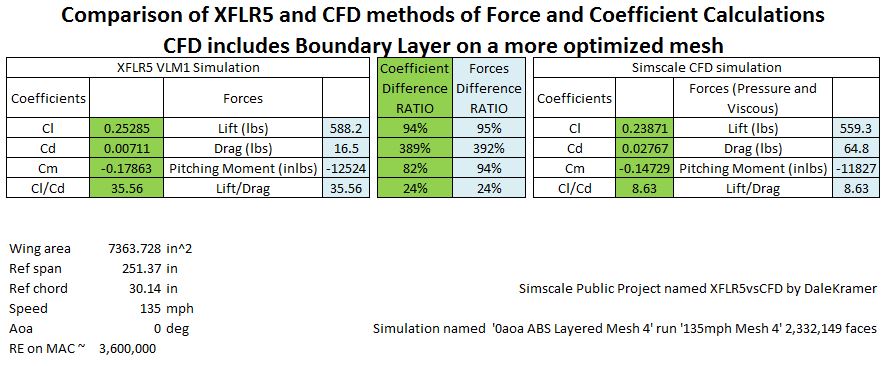
And here is the XFLR5vsCFD SimScale project the chart data came from.

Here is a link to Post 1 where you can see where this chart started life and there is a link there to get you back here quickly…

1 Like

Wow, now that we have a more valid layered mesh and its output data added to the chart… Phew …

I put a note at the beginning of Post 1 to try to reorganize this Topic.

Here are the questions from my first post that are still basically unanswered:

  1. What is most likely the cause of that BIG difference between Cd’s?
  2. Why did the CFD simulation complete with an error (Re Post 1 ‘CFD does NOT include Boundary Layer’ Table)?
  3. Which CFD case is closer to reality (including Boundary Layer or Not)?
    6: If CFD results really are closer to reality, why is good old XFLR5 Lift/Drag ratio so far off?

Anyone care to take a shot at them now? :upside_down_face:

Thanks,
Dale

1 Like

This is where CFD is most useful, we can slice the fields for pressure and velocity through the wing and see why. Create a velocity and pressure slice for with and without boundary layers, furthermore, if you want to invest time into learning to use paraview you could create a delta plot to visualise the difference between the layered and no-layer model (this is not easy though).

Not really sure, can you explicitly send me a link to that project?

Just one thing, be careful about terminology, if the walls are no slip there will always be a boundary layer, and if we are modelling with wall function a certain part of that boundary layer will be modelled. The statement should be with or without cell layer inflation, where with inflation, modelling will likely be correct, without it would likely be incorrect. So with wall inflation is likely to be better. With no validation, however, we can simply say that considering all best practices appear to have been followed, results are likely to be accurate.

I don’t know I am afraid, sorry.

Best,
Darren

2 Likes

Darren @1318980

Excellent answers! :+1::+1:

I may just do that when I have some time (interpreted as not in the foreseeable future :wink:, but oh-oh I see another forum topic :smile:

Sorry, simulation was renamed after I started playing with expansion ratios. It is still in the [original project][Deleted by author], Simulation named ‘ExpRatio1.3 Layered and Refined mesh 2’, Run named ‘ExpRatio1.3 135mph’. The Force and Coefficient Plots stop at ~250s and are very stable before 250s. The Convergence Plot stops at ~90s but ‘looks like’ it would converge at or before 250s.

I will be more careful. I suspected there was some BL formula being used with no cell layer inflation as in that case surface mapping of U, shows 0 everywhere. I just was never able to get an image that showed how it got from 0 to freestream magnitude near the surface.

I guess it really was just a rhetorical concluding question. As you can probably tell by how much burning of the midnight oil has gone on around here, I am sold on SimScales interface with OpenFoam and CFD in general. I guess I have to go back to XFLR5 and do some digging, I will report if I find an error in my case there…

If you are ever in central Florida I have this :rainbow::palm_tree::pizza::cocktail: waiting for you…

Thanks a bunch,
Dale

Is there a way to set up a simulation to assume irrotational flow?

I found this SimScale Doc that suggests a Potential Flow Analysis is what I want, but I have not been able to figure out from that link what parameter values are actually needed to set up a Potential Flow Analysis. It is a great link that provides a lot of parameter explanations but not to tell me what to do to set one up and it looks like it MAY be 2D.

And then I thought, aha, I bet if I just did a laminar simulation, it would be irrotational and then I find out not all laminar flows are irrotational :frowning_face:

Just trying to be able to compare apples to apples as it looks like XFLR5 assumes irrotational flows.

Thanks,
Dale

:smiley: cheers buddy sounds amazing!

Great I’ll check this out and get back to you.

Yes, that is what you are looking for, and unfortunately, it was removed as analysis type because nobody used it and it wasn’t accurate in most cases anyway. All is not lost, however, if you go into simulation control and select initialise with a potential flow (it might already be set as true?) then the time step 0 will have the results of the potential flow simulation (we use it to get a better set of initial conditions). The catch is, that I am not sure if lift and drag values are reported for 0-time step, if so great, else, you might have to do some imaginative post-processing in paraview.

Also, I read a paper showing that in 2D cases lift and drag values for both Blade Element Momentum Theory and CFD both showed to have a similar lift and drag values and were similar to experimental also, now, it could be that the CFD model could be run through a mesh independence study to get more accurate results, but I would not have said that the level of indifference could be corrected. My theory is that a 3D BEM doesn’t solve things like lift-induced drag caused by tip vortexes and the like, however, at this moment cannot find a paper to back it.

If I had to do what you are doing, I would be tempted to go 2D, not because it is what I want to simulate, but because it would prove to myself that the setup is valid and that CFD does agree with xfoil, and if so, move on with the assumption that the 3D results would also be correct. This is because, despite apparent simplicity, wings are not easy things to simulate, and if sufficient mesh is not present where needed, then this could skew results. And knowing what the results should be, compared to CFD, we can easily determine what is working and what isn’t, at this moment in time, both BEM and CFD could equally be valid, we just don’t know :slight_smile:

Good luck,
Darren

1 Like

Ok, there is no reason why this error happened, it looks to me like it just crashed, I will report this issue immediately, but for now please just restart the simulation, and most definitely let me know if it occurs again (I think it would be unlikely). Also, if I was selecting an instance to run on, I would probably pick a 16 or 32 core machine for a 3 million cell mesh, to be efficient but your choice :smiley: might be worth checking you are actually saving time though.

Best,
Darren

Thanks, that simulation was eons ago in my 15 day learning curve :upside_down_face:, I have since learned a lot from different sources on # of core usage. In my memory now is #volumes/50,000 if #volumes < 500,000 else /100,000, whats your in brain memory formula? :wink: Also, what is in your memory for what to remember most about a mesh, nodes, faces or volumes?

Ahah, I don’t actually have a formula, I just tend to band into 3 categories, sub 1 million sub 16 cores, 1-5 million 16-32 cores, more than 5 million 16 core + depending on ram needed and how fast I want the results :smiley: But that’s me just being lazy.

I remember volumes, I normally say mesh size, by that I mean size in terms of cell count. So 500k and 32 million, would be mesh sizes to me in terms of cells/volumes.

Best,
Darren

1 Like

Like that post for sure, now that is GOOD info!!! :smile: :smile: I’m coming from 3D printing closed surface meshes and I think ‘faces’ about them…

Ok, you are starting to convince me :wink:

In the meantime I tried a laminar flow assumption on the NON layered mesh with air viscosity 0 (I was trying to stop rotation) but that only got the Cd by CFD to be only 320% bigger than XFLR5.

I will try the 0-time look at NON layered mesh with potential flow initializing and report back.

2D is next :wink:

BUT for sure my eyes are opened and are seeing for sure why XFLR5 type programs should not be relied on for real life 3D situations about drag…

Sorry Daren but I do not see anywhere to set up a potential flow initialization. Where to find?

I looked in ‘Initial Conditions’, ‘Velocity Inlet’ of ‘Boundary Conditions’ and just about every less obvious place :slight_smile: .

Also, would you suggest Laminar as turbulence model?

What do you think of making the walls on the geometry as slip walls?

I have not found a quick way to check cores hours for a mesh and simulation, are they just listed at the end of the Meshing Log (ie Finished meshing in = 29.93 s) and Solver Log (ie ExecutionTime = 578.18 s)?

Hi Dale,

you can find this via your Dashboard when you go to the top right drop-down menu clicking “Manage Account”. There you can see every project with the amount of core hours used.


Is that what you wanted to see?

Jousef

I have looked at that in the past but have not been able to see what I did, right after I do it.

Also, is was sorted weird as a default.

Then when I sort by start time, at this current the last operation shows as ‘2018-08-03 9:41:37AM’ while my current time is ‘2018-08-03 7:04:02PM’ . It seems way too dated for my use.

My Dashboard under ‘Latest jobs’ says I last did a job at ‘Start: 8/3/2018, 12:39:07 PM’ which is likely correct, but there I can not see core hours.

I would like an instant way of seeing core hours preferably in the WB for meshing and simulations.

Dale