XFLR5 vs CFD

But I had the impression that these ‘layers’ we add to the mesh was the region where the speed of the air particles changed from 0 at the no-slip surface right up to the local freestream speed based on some rate of change curve set by the turbulence model, sort of like the boundary layer…

True, and the distance from the surface to the dimensionless distance to the first layer from the surface is the Y+ value you are observing here. However, wall modelling is only valid in the log region of the boundary layer, which is why, it is recommended to get the value between 30 and 300, as here the boundary layer is extremely predictable. bellow 30 there is the buffer layer and the linear layer, where if we fall in this region and model logarithmically it will be incorrect, likewise, as we start moving away from the wall above 300 there is increasing deviation from the log law. So the Y+ distance takes into account the distance to the first cell (Y) and the surface friction in relation to the U+ which is the dimensionless velocity, this is how wall modelling works. It works great as long as we obey its requirements.

Does that make sense? so in order to predict the correct conditions at the boundary of the first cell using a logarithmic relation we need to ensure the cell distance lies in that logarithmic region.

1 Like

It is clearer but still confusing, I am sure at some point I will have an AHA moment and feel comfortable with it.

I just can’t get a handle on why the overall thickness of these added layers vary with their original mesh cell size, the actual boundary layer doesn’t change thickness because some mesh algorithm decided that an area needs a finer mesh. But if you say the math works out regardless that these added layers vary in thickness over areas where the true boundary layer does not, then I believe you.

From what I can tell at this point, I want to try to get the yPlus value to average ~165 at the surface of the geometry. To determine a surface average, I can do surface mapping as in the above images and set a yPlus color range so that my eyeball tells me what the surface average is for the surface in view.

This seems very cumbersome, why can’t the postprocessor just let me select a surface (or my whole geometry) and then tell me what the yPlus, max, min, average, std deviation etc. values are for that surface?

I also assume I want the mesh slices in the mesh result to actually SHOW the 5 or x number of layers added in the layering process. So why are the mesh layers ‘missing’ in the middle image of my last 3 images (and actually it was over the whole wing as far as I can tell, not just near the trailing edge)?

Very good suggestion and I agree entirely. Please, can you add this suggestion into our vote for features part of the forum?

There are a lot of quality checking that goes on in snappy hex mesh, and it does take a bit of experimenting to get this correct. For example, the volume ratio of the two cells might be too high so the algorithm cancelled inflation, this could be solved by reducing the expansion ratio or by increasing the allowable volume ratio.

Counter-intuitively maybe, increasing the expansion ratio will actually reduce the Y+. This is because the algorithm is maintaining a final cell size and adjusting the lower ones to be thinner. A better method would be to just reduce the number of cells, and if this doesn’t work we could use full resolution modelling (better suited to smaller Y+ values of around 1).

1 Like

Done, as long as you will vote for it :wink:

Darren @1318980,

I have been working hard trying to get the best mesh to start with before I layer the wing.

I have started a new public project with what I have done so far.

There is one geometry and two meshes in the project so far but I am working on the project and may try a simulation soon.

Mesh 1 is just a refined geometry with 2.03 million faces.

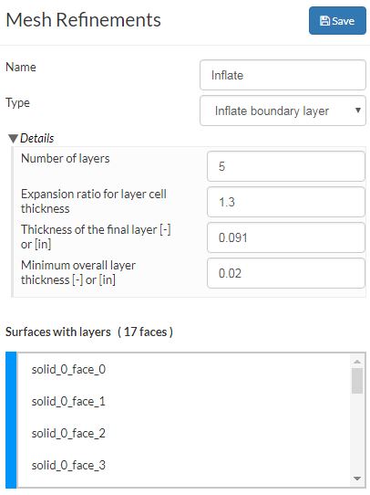
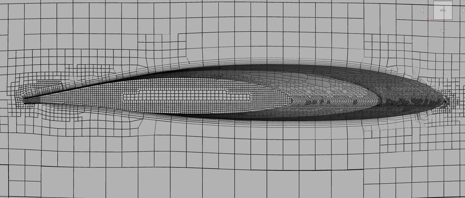
Here is Mesh 1 near the wingtip (~12 in chord and 0.17 in TE thickness) :

The 3.02 million face Mesh 2 is my attempt at layering Mesh 1 with the following procedure.

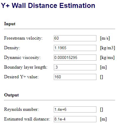
I am using the ~12 in tip chord and 135mph in the yPlus calculator like this:
yPlusforXFLR5vsCFD

Then in a spreadsheet I have this:
ParaCalcsFromEWD

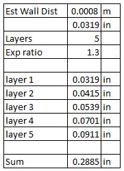
Then in Mesh Refinement Parameters for Inflation I did this:

Then I started clipping Mesh 2 to view the layers I added to Mesh 1. I am not sure if they are good enough and don’t know where to start to make them better. I do not see an ‘allowable volume ratio’ in the Parametric parameters and I am a little confused about your other suggestions.

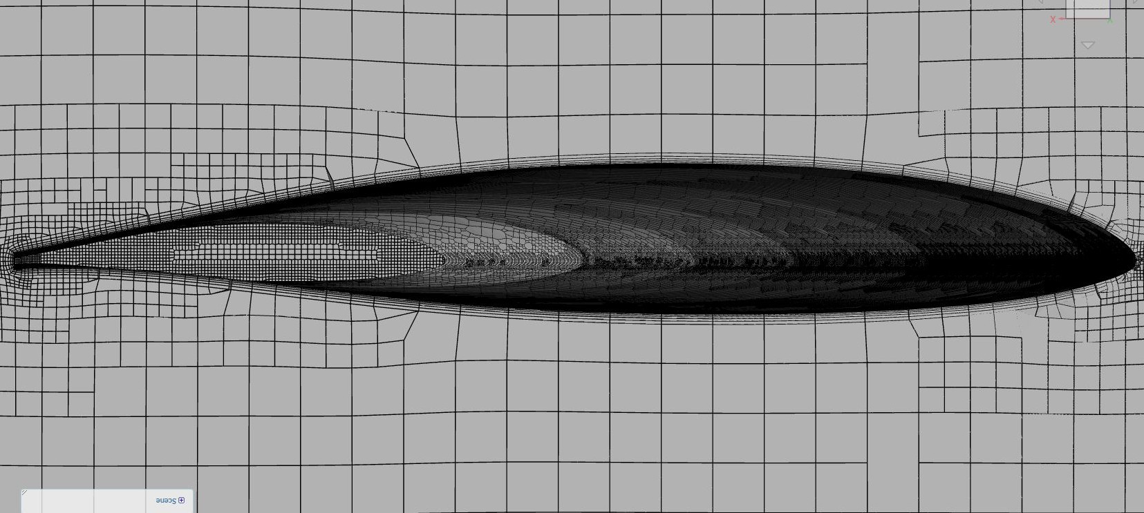
Here are the mesh clips, first, right at the wingtip:

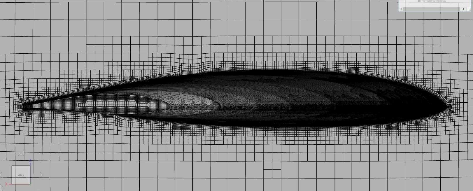
6 inches in from tip:

At 1/2 span:

And at the root:

Can you give me any specific pointers to refine the layers now so I can go on and make a 1s simulation to see if I got the average surface yPlus anywhere near the 160 that I want?

Thanks,
Dale

1 Like

I did run a 1s simulation and I am very dissappointed that the yPlus at the surface seems to only average about 2.

What did I do wrong?

yPlus plots (yPlus [point_data]):

yPlus Bottom:

Time to go to bed :upside_down_face:
Dale

EDIT: Strange, this morning I wake up and decide to ‘save a state’ with my setup to view yPlus but now I can only achieve a view that shows the average yPlus is about 1 (not 2 like last nights images :disappointed_relieved:). Do I have the ‘saved state’ setup up properly this morning to view Yplus (I think it is too much of a coincidence that the average is 1, am I looking at some sort of Normalized value now)? Maybe I am just too groggy this morning :upside_down_face: :

Here is a mesh clip at y=-37.7 which is the start of the first wing planform taper and where the first big red area is (any way to fix these red islands, you can see the lack of layers there in this image):

The overall Layer thickness wherever they actually get added is about 0.3 inches, so the Parameter input looks OK, just why is the yPlus average showing at 1, and not 160?

Darren @1318980,

Now this is worth a new post…

So I look at the top planform view of the Mesh 3 at the y=-37.7 start of planform taper into another surface and I have an AHA moment:

As you probably know I have an active Topic about 2 issues I am having with Feature and Surface Refinements.

The cause of the yPlus discontinuities in the above image is Issue #2 at this post. I do not think the layering algorithm can handle that angular jaggy causing the layers to deflate there.

The mesh jaggies at this surface/surface edge intersection as seen above are Issue #2 exactly. I have tried to reduce the effect of Issue #2 in my mesh by simply refining all the way to Level 11 (overkill I think but had to due to Issue #2). Unfortunately, there are still jaggies even at Level 11 and this is one of them, If I go to a Feature Refinement these ‘step changes of leading edge planform angles’ at the wing ‘ribs’ will also be refined at Level 11 but at a cost of a larger mesh size (a temporary solution at best until Issue is fixed :wink:).

Also, if you look closely at the leading edge joint in the mesh, even at Level 11 there is still small jaggies, which I believe is causing a lot of the small leading edge red zones in the yPlus planform mapping.

I will try the bandaid Feature Refinement and report back…
Dale

Hi @DaleKramer, there is a lot of info here, I just wanted to comment that the red zones that show higher Y+ might actually be where the layers cancel:
8767fe25a7e792b97f1a44504420de50c04d1742_1_690x304

And on the topic of jiggles :slight_smile: Not sure what is classed as a jiggle, but there will always be some geometry miss representation, we just make the mesh finner until the representation is sufficiently close.

Also on the Y+ estimation and actual, did you turn relative layers off? I have always found that there is some difference between estimation, with some estimates being very off, but they are useful for getting a starting point, and then with results altering the mesh until the correct y+ values are obtained.

Best,
Darren

If you have a surface highlighted or selected on a mesh and you look at the edge faces, a ‘jaggy’ is where any outside edge face has outside edge corner points that are not precisely on the geometry edge curve which the mesh surface should be following.

I understand that you look at this as just a miss representation which is ‘fixed’ (but not really, you just get smaller jaggies) by meshing finer but that is a bandaid solution. There should be ZERO jaggies on a Surface or Feature Refinement whose job it is to follow the geometry edge curves.

It appears that the layering algorithm can handle what I call Rectangular Jaggies but not the Weird Angular Jaggies where the yPlus red zones are:

Yes relative layers are false.

The the expected yPlus of 160 is SO different that what I got of 1 or 2 depending on which time I viewed yPlus :slight_smile:

I try to use jag… vs jig… because a jiggle to me is a motion shake and a jaggy is like the jagged edge of something :upside_down_face:

Oh if I could only figure out what layer or mesh parameter to change to stop these dips from happening on my layers (that is a ‘rib’ location with Feature Refinement to Level 9 to reduce the jaggies):

I would be in heaven :rainbow::palm_tree::pizza::cocktail:

@DaleKramer, so we got a mesh, that I would say is acceptable, we could go with this mesh, there are lots of settings in the mesher that will alter this but I’m not sure it would significantly affect results. I would try reducing this to maybe 1 or 2 inflated cell layers and then run with full res and wall modelling to determine the result change. if none, then we probably have good results. Could we then compare to experimental data? is there any?

Best,
Darren

Edit:
We could simplify this to a wing section, validate the results and once valid we can assume the full wing will also be valid?

Darren @1318980

Making progress…

I was able to get a pretty decent layering (and I am sure I can do better, will explain what I did after I refine it a little more) but I ran into some issues trying to see the relevant yPlus Range and even issues on what the real range is after I did a Save State.

Remember when I asked if the range was ‘normalized’ somehow, well I think it is because we are looking at the data on the first simulation iteration. I finally had an AHA moment and decided to run it to convergence. That converged range is finally what I was expecting and if I can trust the results from opening the PostProcessor from the Solution Fields, here is the mapping and adjusted range so that I get the most Green area on the wing (I REALLY want those max, min, average, std deviation numbers :slight_smile:) :

I think I am pretty good with everything now but I need to wait on my new topic results before I am comfortable with presenting more data here…

I may carry on under the premise that something is not right with the presentation of the data AFTER the saved state gets the data…

What do you think?
Thanks for all the help.
Dale

P.S. :grinning::grinning::grinning::grinning: Check out my post 21 here, I think I have found out that Save State issues may be the culprit on that one, not my groggy 4:00 am brain…

I don’t really have experimental data, just XFLR5’s predictions which I know are not quite realistic even though it is based on sound methods.

I really don’t want to simplify the example too much, I am sure there are many comparisons of section data with CFD already. I do not necessarily want to have to rely on an assumption that a full wing would be valid.

Dale

Well, here is about the best I could do.

For the Inflation parameters, I’ve got 3 layers, 1.1 expansion ratio and a 0.03821 in. final layer.

There is still a small deflation on the top of the wing and 3 larger ones on the bottom.

But I think by looking at these images and except for the deflations, we can say I have yPlus generally between 30 and 100.


Now I will make a new Comparison Chart between XFLR5 vs CFD and add it here in the morning along with a synopsis of how I meshed the wing within the limitations of the current refinement algorithms (Mesh 4 in the project is the best and it currently has 2,300,000 faces including the layering).

Dale

And my current meshing strategy is (I update this as I learn more :wink:) :

  1. Decide on the wind-tunnel wall sizes and location of the geometry in it, then define these in the Background Mesh Box coordinates. For me, that BMB (on my left/right symmetrical geometry), was about double the wingspan wide, centered in triple the height of the geometry (but much more for just a wing and more if at high aoa’s) and with a BMB length 4 times the length of the geometry with geometry positioned one geometry length back from the front of the BMB.
  2. Set Parameters for number of x,y,z cells on the Background Mesh Box (I started with about ~50 inch mesh squares, it is these cells that get divided by mesh refinements on the geometry. BUT, in the end, 15 inch squares were best for this 125 inch half span wing based on final BMB dimensions and final refinement levels chosen)
  3. A wing geometry should have 3 spanwise edges, 1 at the leading edge at the smallest radius of the airfoil and 2 at the trailing edge. The multi taper wing was split into spanwise planform taper surfaces with ‘rib’ surface edges at each change in taper. You can not have intersecting solids in your geometry, so far I boolean all my touching solids together into one solid in CAD but I expect later to use multiple touching solids but that do not intersect. So far I have only used solids, but I understand that single surface meshes and closed meshes can be used but likely with the same touching/intersecting rules.
  4. You might have to create a narrow surface break near the plane of symmetry to get Surface refinements to act on the symmetry edge of some surfaces (you may likely only have to do this if your geometry is already a 1/2 model of symmetrical item).
  5. I use a cartesian box to provide a refinement ‘outside’ the geometry that is refined at level 2 so that the air gets ready to hit the geometry in smaller cells. I am using about 1/2 the length of x,y and z dimensions of BMB and positioned sorta like the BMB is positioned around the geometry.
  6. I use a cartesian box to enclose the geometry pieces (ie Wing, Horizontal stabs, Fins, Fuselage) and create a Region Refinement for all of them at a Level 5 refinement level.
  7. I used a Surface Refinement on all the wing surfaces to try to get all the edges of the surfaces clearly defined in the mesh. I had to go to Level 10 fineness to minimize the effect of edge jaggies and to keep the trailing edge defined all the way to the wingtip. Unfortunately, I had to change the Level back to 8 when I started layering the mesh since the layering algorithm was choking on the small face sizes and deflating everywhere, so the level was a balance between edge sharpness and layering results.
  8. To keep total number of faces low, I set the edge distance of the Surface Refinement to 0.
  9. Set layering variables to match your needed yPlus, reference length and speed. Here is where I finally figured out how to do this.
  10. To determine if my layering has succeeded sufficiently, I no longer look at clips of my mesh (very tedious). I just use my method of getting a weighted % inflated value for the mesh from the last % inflated chart in the meshing log. This post should show how to create the weighted % inflated mesh parameter.
  11. To get my yPlus between 30 and 300 without too many layer deflation zones, I am using only 2 layers at an expansion ratio of 1.1 or 1.2. I use the old post processor to look at my yPlus range on the on a surface plot of yPlus onto the geometry (this is done on the results of a CONVERGED simulation). The old post processor lets you turn off the bounding box and internal mesh to do this and I can’t figure out how to do the same in the new post processor.
  12. Make sure Parameter ‘Use relative size for layers’ is off (false).
  13. Add Darrens Tweaks (see this post)

Someday when I have to do this again, I will be coming back here to remember what I did :wink:
Dale

And here is the new comparison chart, I am still surprised that the CFD drag is reported as nearly 4 times the XFLR5 drag.

And here is the XFLR5vsCFD SimScale project the chart data came from.

Here is a link to Post 1 where you can see where this chart started life and there is a link there to get you back here quickly…

1 Like

Wow, now that we have a more valid layered mesh and its output data added to the chart… Phew …

I put a note at the beginning of Post 1 to try to reorganize this Topic.

Here are the questions from my first post that are still basically unanswered:

  1. What is most likely the cause of that BIG difference between Cd’s?
  2. Why did the CFD simulation complete with an error (Re Post 1 ‘CFD does NOT include Boundary Layer’ Table)?
  3. Which CFD case is closer to reality (including Boundary Layer or Not)?
    6: If CFD results really are closer to reality, why is good old XFLR5 Lift/Drag ratio so far off?

Anyone care to take a shot at them now? :upside_down_face:

Thanks,
Dale

1 Like

This is where CFD is most useful, we can slice the fields for pressure and velocity through the wing and see why. Create a velocity and pressure slice for with and without boundary layers, furthermore, if you want to invest time into learning to use paraview you could create a delta plot to visualise the difference between the layered and no-layer model (this is not easy though).

Not really sure, can you explicitly send me a link to that project?

Just one thing, be careful about terminology, if the walls are no slip there will always be a boundary layer, and if we are modelling with wall function a certain part of that boundary layer will be modelled. The statement should be with or without cell layer inflation, where with inflation, modelling will likely be correct, without it would likely be incorrect. So with wall inflation is likely to be better. With no validation, however, we can simply say that considering all best practices appear to have been followed, results are likely to be accurate.

I don’t know I am afraid, sorry.

Best,
Darren

2 Likes

Darren @1318980

Excellent answers! :+1::+1:

I may just do that when I have some time (interpreted as not in the foreseeable future :wink:, but oh-oh I see another forum topic :smile:

Sorry, simulation was renamed after I started playing with expansion ratios. It is still in the [original project][Deleted by author], Simulation named ‘ExpRatio1.3 Layered and Refined mesh 2’, Run named ‘ExpRatio1.3 135mph’. The Force and Coefficient Plots stop at ~250s and are very stable before 250s. The Convergence Plot stops at ~90s but ‘looks like’ it would converge at or before 250s.

I will be more careful. I suspected there was some BL formula being used with no cell layer inflation as in that case surface mapping of U, shows 0 everywhere. I just was never able to get an image that showed how it got from 0 to freestream magnitude near the surface.

I guess it really was just a rhetorical concluding question. As you can probably tell by how much burning of the midnight oil has gone on around here, I am sold on SimScales interface with OpenFoam and CFD in general. I guess I have to go back to XFLR5 and do some digging, I will report if I find an error in my case there…

If you are ever in central Florida I have this :rainbow::palm_tree::pizza::cocktail: waiting for you…

Thanks a bunch,
Dale