Recording

Homework submission
Submitting all three homework assignments will qualify you for a free Professional Training (value of 500€) as well as a certificate of participation.
Homework 1 - Deadline 13th of October, 12pm
Exercise
Have you ever thought that what exactly will happen to the jet engine if one of the fan blade breaks out? It will rather produce vibration due to overall change in center of gravity of a jet engine. But how much it will vibrate? In this exercise we will be looking in to the similar vibration of the jet engine due to blade loss.
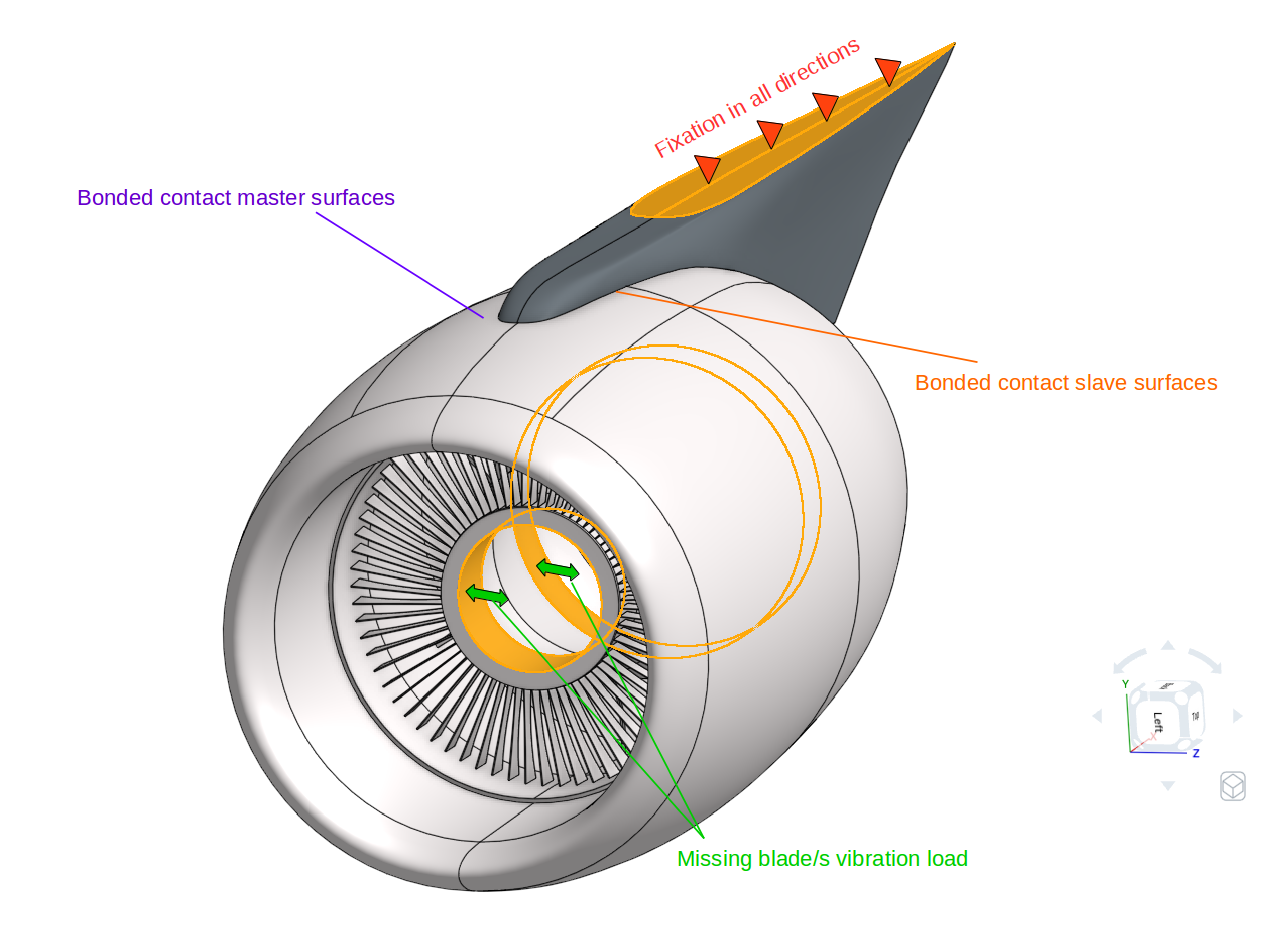
The cutout of the jet engine geometry used in this exercise is shown in the figure below. Only the outer cowling (with strator and struts) and pylon are taken for this analysis, whereas the internal whole jet engine and wing will be ignored since we are only interested in the impact of its vibration on to the cowling via strator and struts.

-
The base model for whole assembly except the internals of jet engine is provided by Aisak from GrabCAD.
-
The base model for the internals of jet engine is provided by Goutam Das from GrabCAD.
This exercise focus on the vibration study of the jet engine cowling due to missing single or multiple fan blades. First, a frequency analysis will be performed in order to get the natural frequencies of the the model. Next, harmonic analysis will be performed on a specific frequency range of interest with the missing blade vibration load in order to see at which frequency the vibration will be highest. Harmonic analysis produces a sinusoidal load through which one can detect the peak displacement value at specific frequency. The model with missing single and multiple blades are shown in the figure below.

Jet engine assembly with 1 missing blade

Jet engine assembly with 2 missing blades
The different combinations for performing the simulations are:
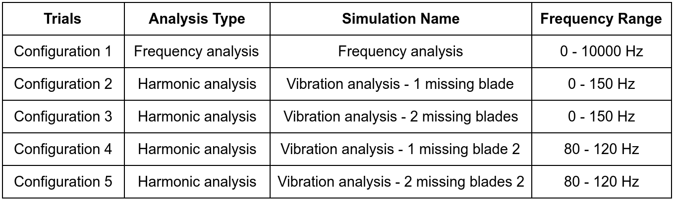
Please note that separate simulation needs to be set up for each configuration
Step-by-Step
Import the project by clicking the link below. (Crtl + Click to open in a new tab)
Click to Import the Homework Project
Meshing
-
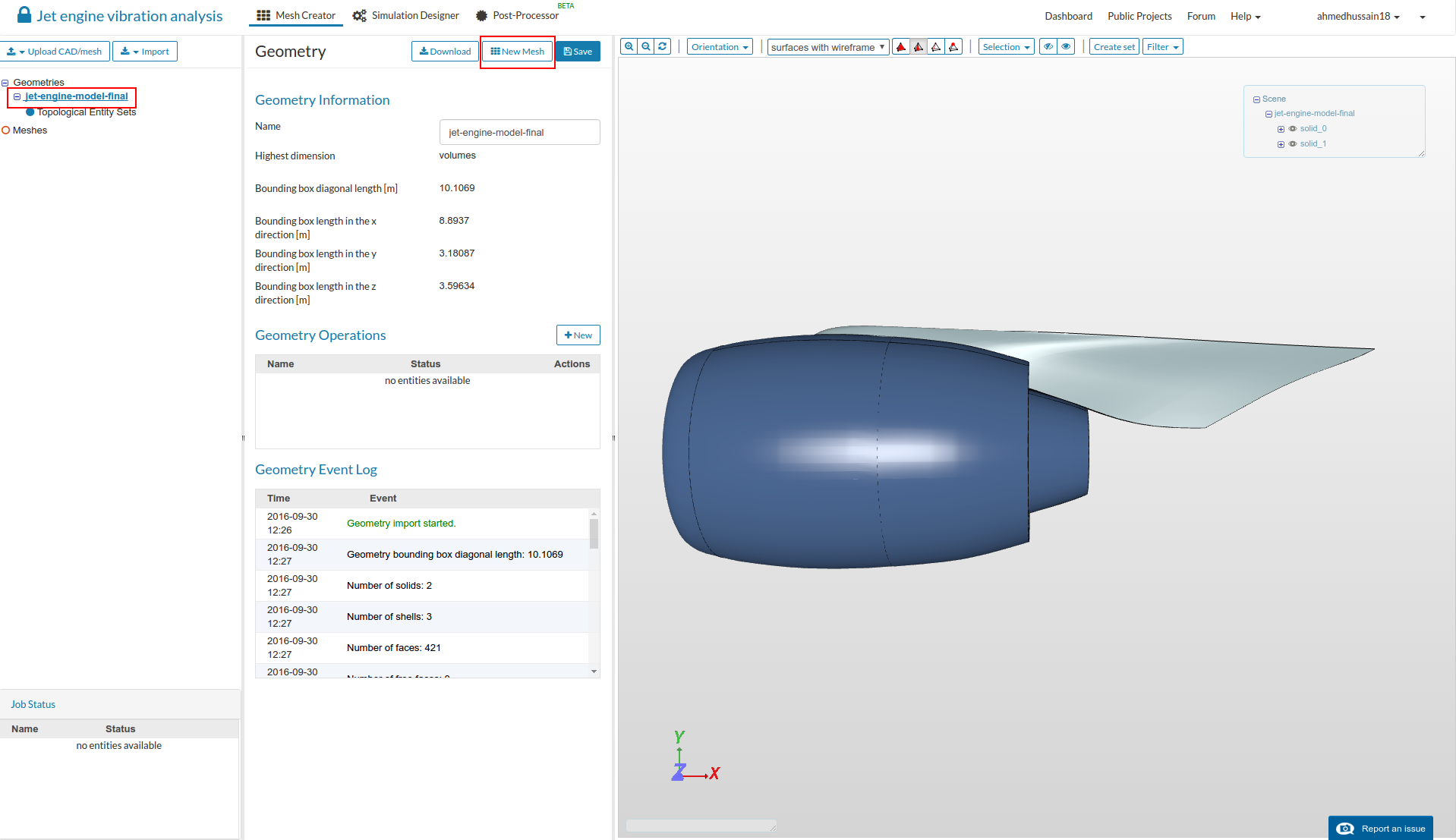
In the Mesh Creator tab, click on the geometry ‘jet-engine-model-final’
-
Then, click on ‘New Mesh’ button in the options panel.
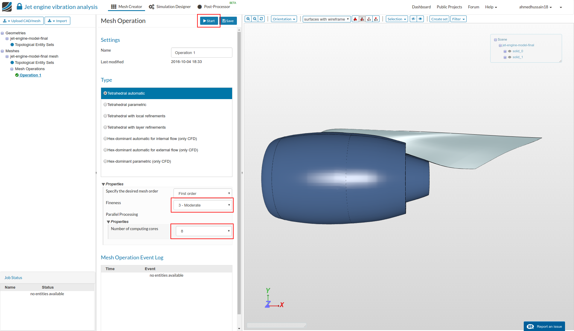
- Change ‘Fineness’ to ‘Moderate’ and ‘Number of computing cores’ to ‘8’. Click on ‘Start’ to start the meshing job. This operation will automatically create a mesh for the geometry. The meshing job will take some minutes to finish and show the status as Finished once done.
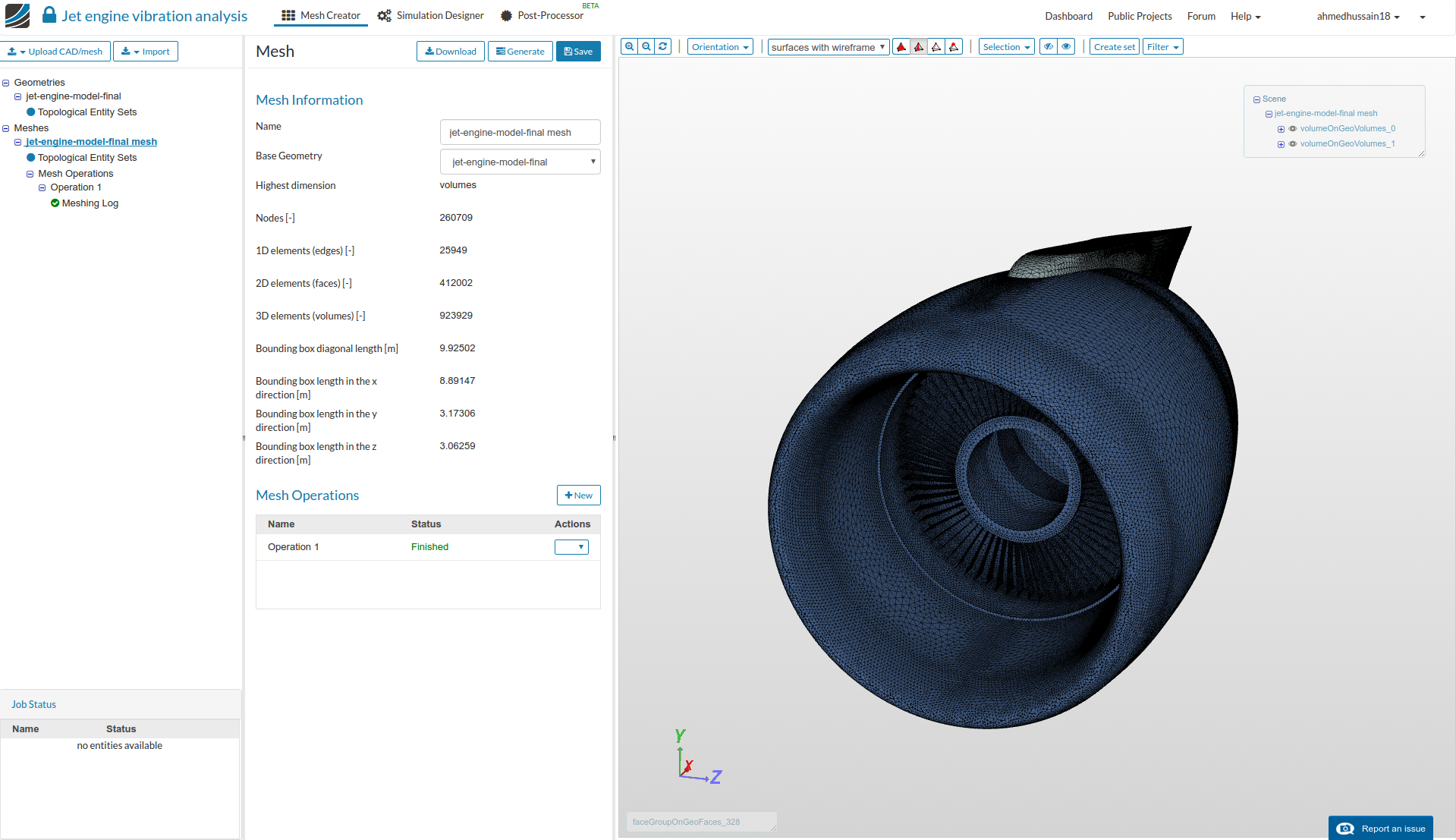
- Once finished, you will see the completed mesh in the viewer.
Simulation Setup
-
For setting up the simulation for ‘Configuration 1’, switch to the Simulation Designer tab and click ‘New’ to create new simulation.
-
A create new project window will pop-up. Give a project suitable name (optional) e.g. Frequency analysis in this case and click ‘Create’.

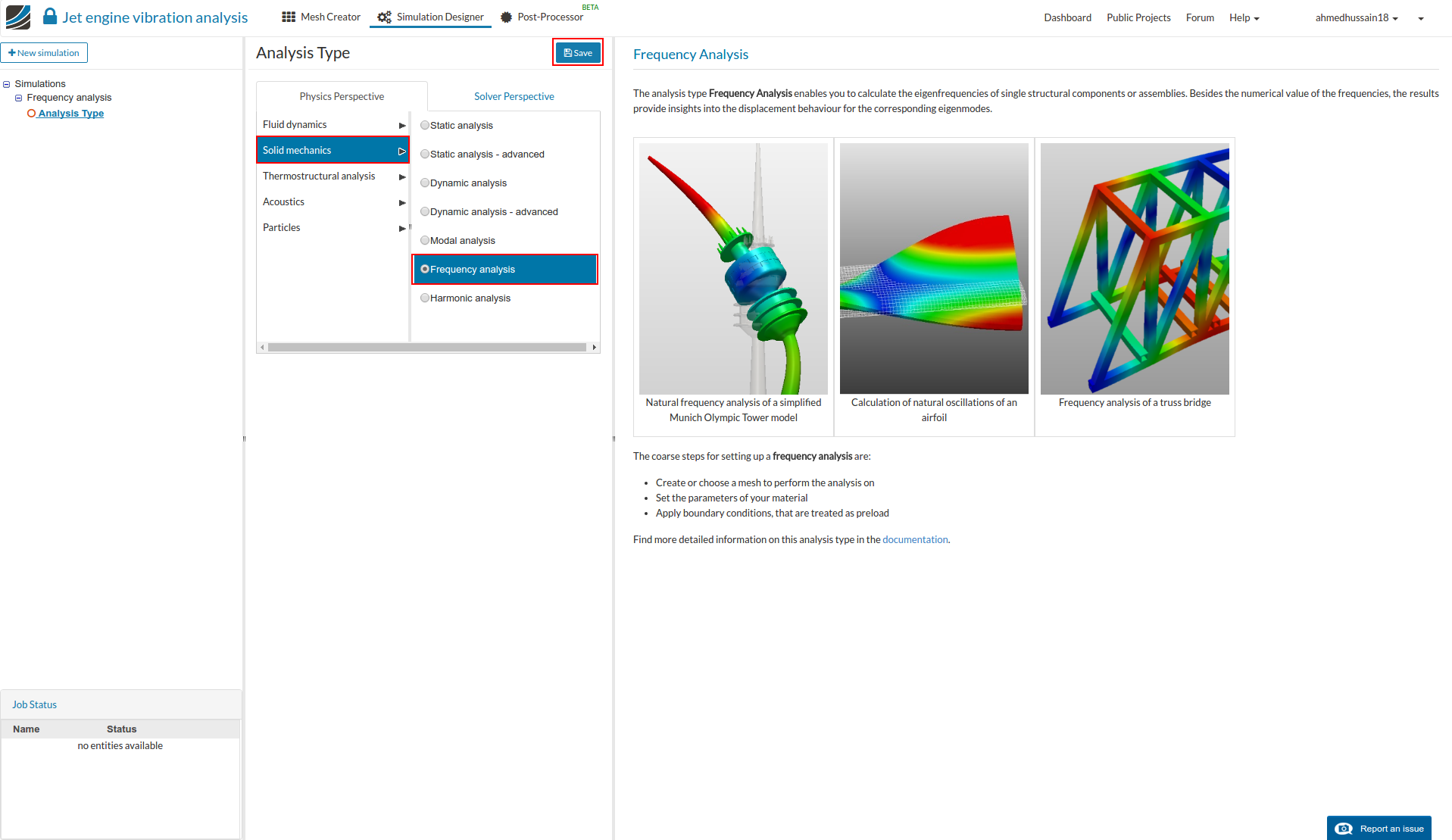
- Select the analysis type ‘Frequency analysis’ under ‘Solid mechanics’ and click ‘Save’.
-
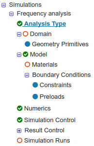
After saving, the simulation tree now looks as shown below. Here the ‘Tree Entries in Red’ must be completed.
Domain selection
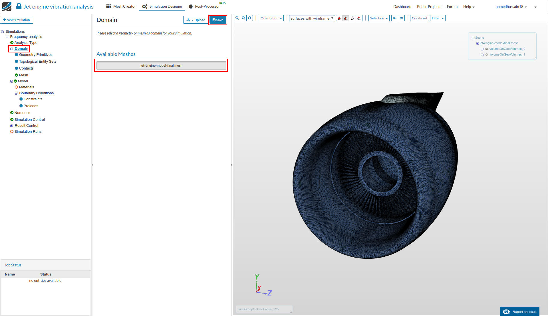
- Click ‘Domain’ from the tree and select the mesh created from the previous task. Click the ‘Save’ button. The mesh will then automatically load in the viewer.
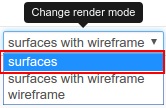
- Furthermore, change render mode to ‘Surfaces’ on viewer top to interact with the mesh more easily.
Topological Entity Sets
- For the ease we will create topological sets in order to use them further in our boundary conditions. The topological sets which we will create will be based on the figure below which explains all the boundary conditions and contact constraints.
- We will create total of 4 topological entity sets as shown below:
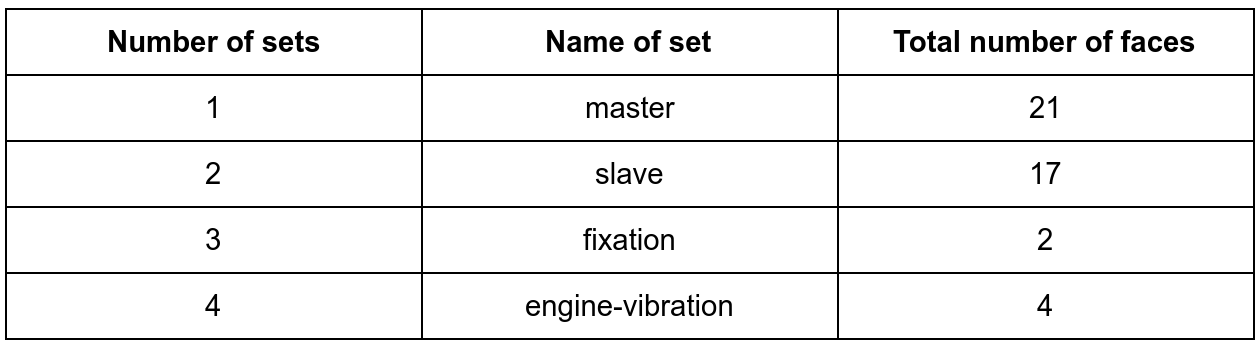
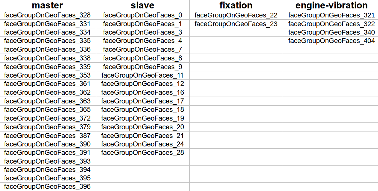
- The faces which will be assigned to each topological set are shown in the table below.
master
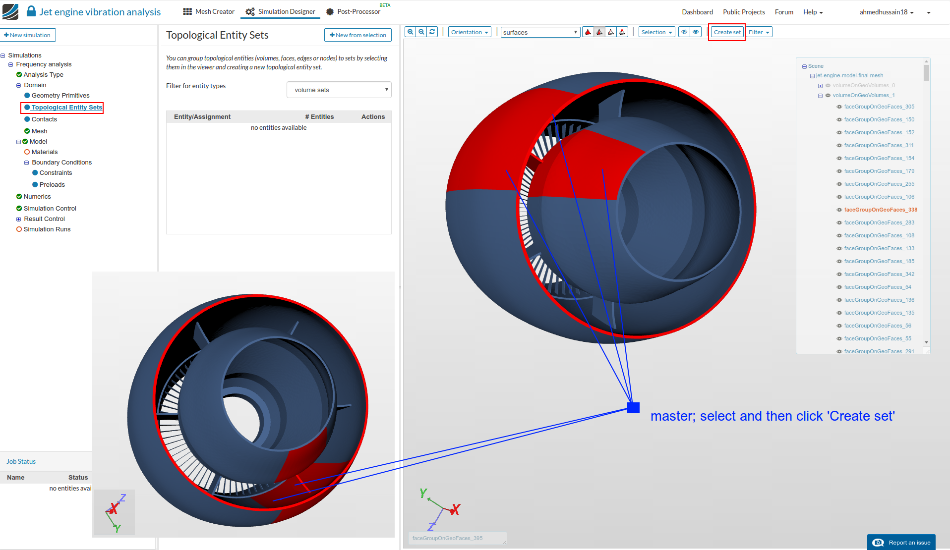
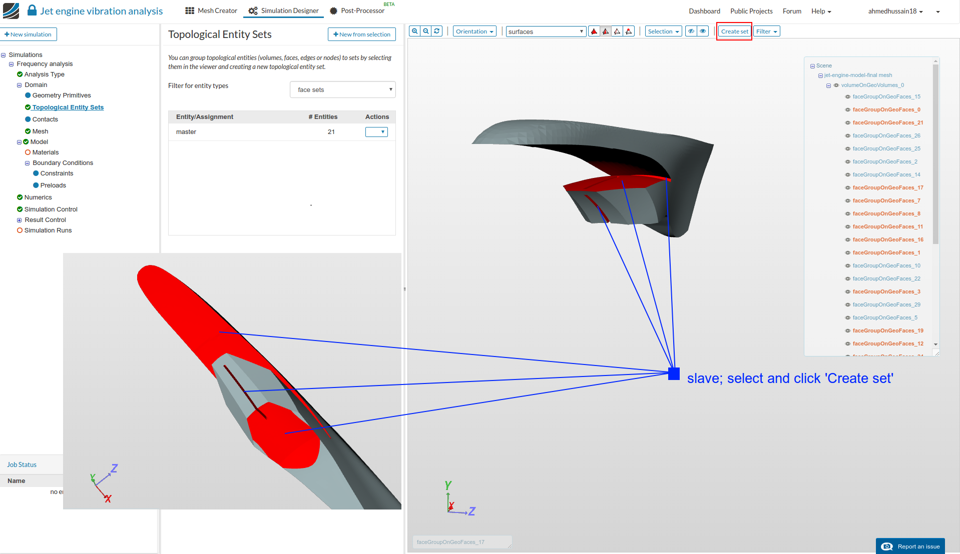
- Go to ‘Topological Entity Sets’, hide ‘volumeOnGeoVolumes_0’ by clicking a small eye icon next to it in ‘Scene’ tree and select all the contact faces of the cowling and strut as shown in the figure below and then click ‘Create set’ on viewer top. Give set a reasonable name e.g. master in this case. Alternatively, you can also select the faces from the right ‘Scene’ tree for ease.
slave
- Follow the same steps as above but this time hide ‘volumeOnGeoVolumes_1’ while keeping ‘volumeOnGeoVolumes_0’ visible and select all contact faces of the pylon as shown in the figure below. Click ‘Create set’ and give set a reasonable name e.g. slave in this case. Alternatively, you can also select the faces from the right ‘Scene’ tree for ease.
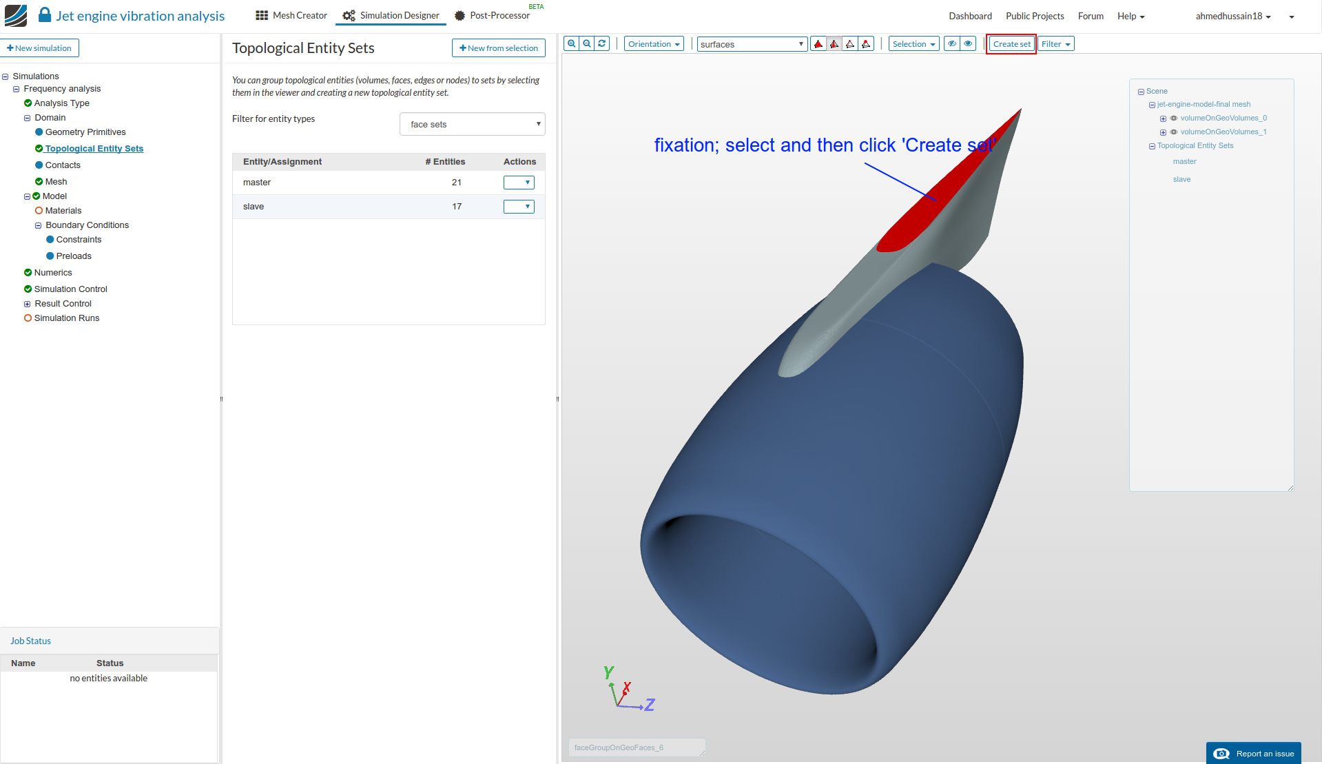
fixation
- Similarly, for the third topological set follow the same steps as above and this time select the upper two faces of the pylon as shown in the figure below. Click ‘Create set’ and give set a reasonable name e.g. fixation in this case.
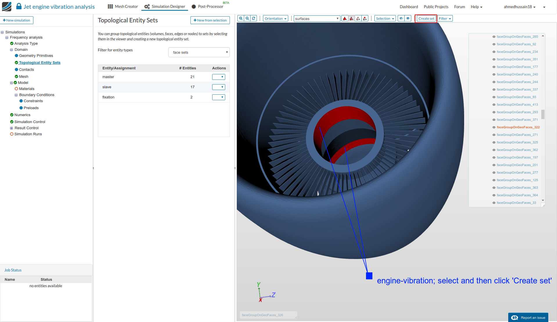
engine-vibration
- For the last topological set follow the same steps as above and this time select the inner round surfaces of cowling as shown in the figure below. Click ‘Create set’ and give set a reasonable name e.g. engine-vibration in this case. Alternatively, you can also select the faces from the right ‘Scene’ tree for ease.
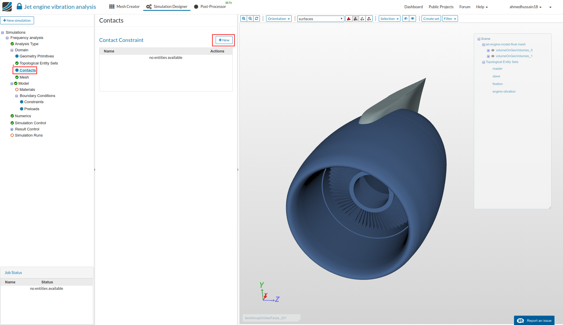
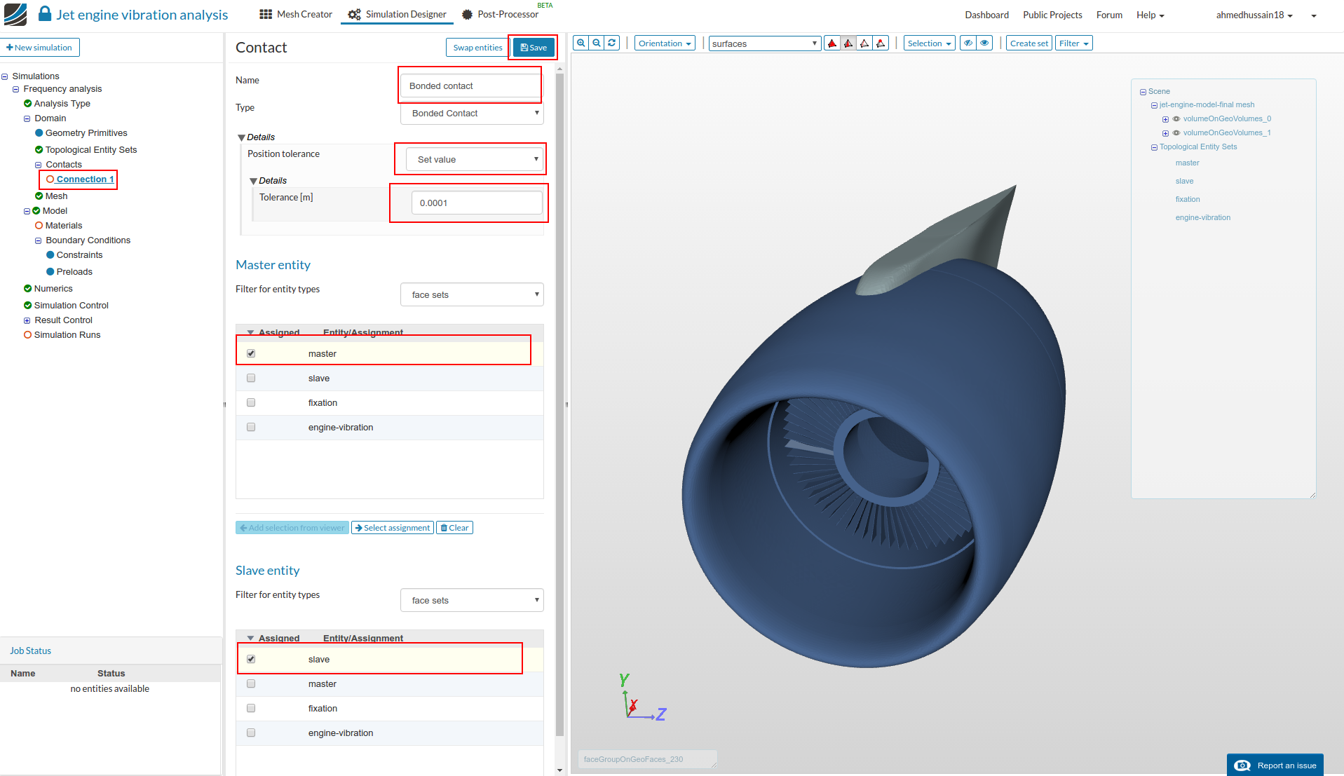
Contacts
- In order to bond the pylon with cowling, we need to define a contact. Go to ‘Contacts’ and click ‘New’ in order to create a new contact definition.
-
Rename the newly created contact to ‘Bonded contact’ (optional).
-
Change ‘Position tolerance’ to ‘Set value’ and then change the ‘Tolerance [m]’ to 0.0001.
-
Select ‘master’ and ‘slave’ under ‘Master entity’ and ‘Slave entity’ respectively. Click ‘Save’ to save the contact definition.
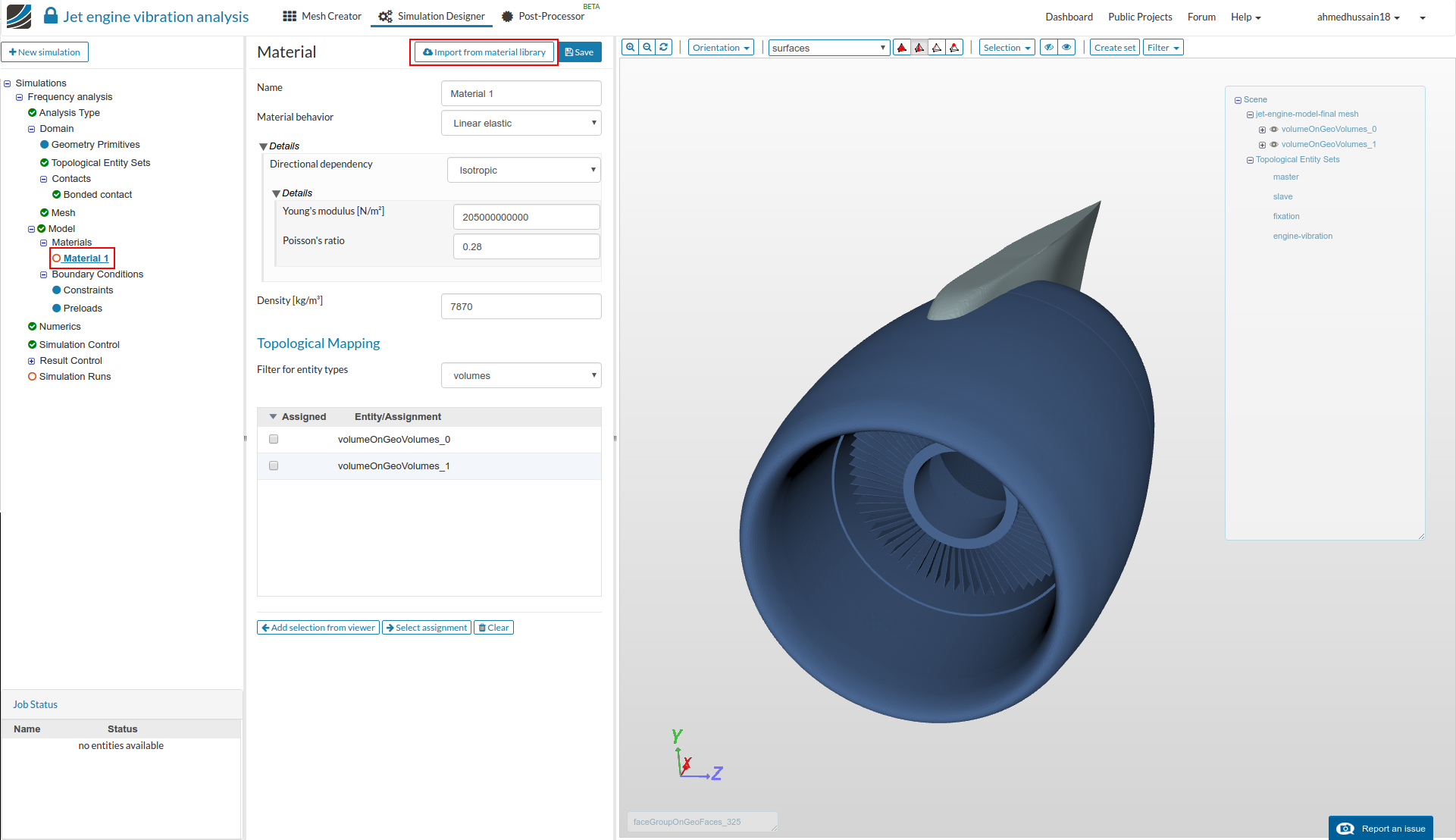
Materials
- In order to define a material, go to ‘Materials’ under tree and click ‘New’ to create new material definition.

- Click ‘Import from material library’ to import the material from the material library database.
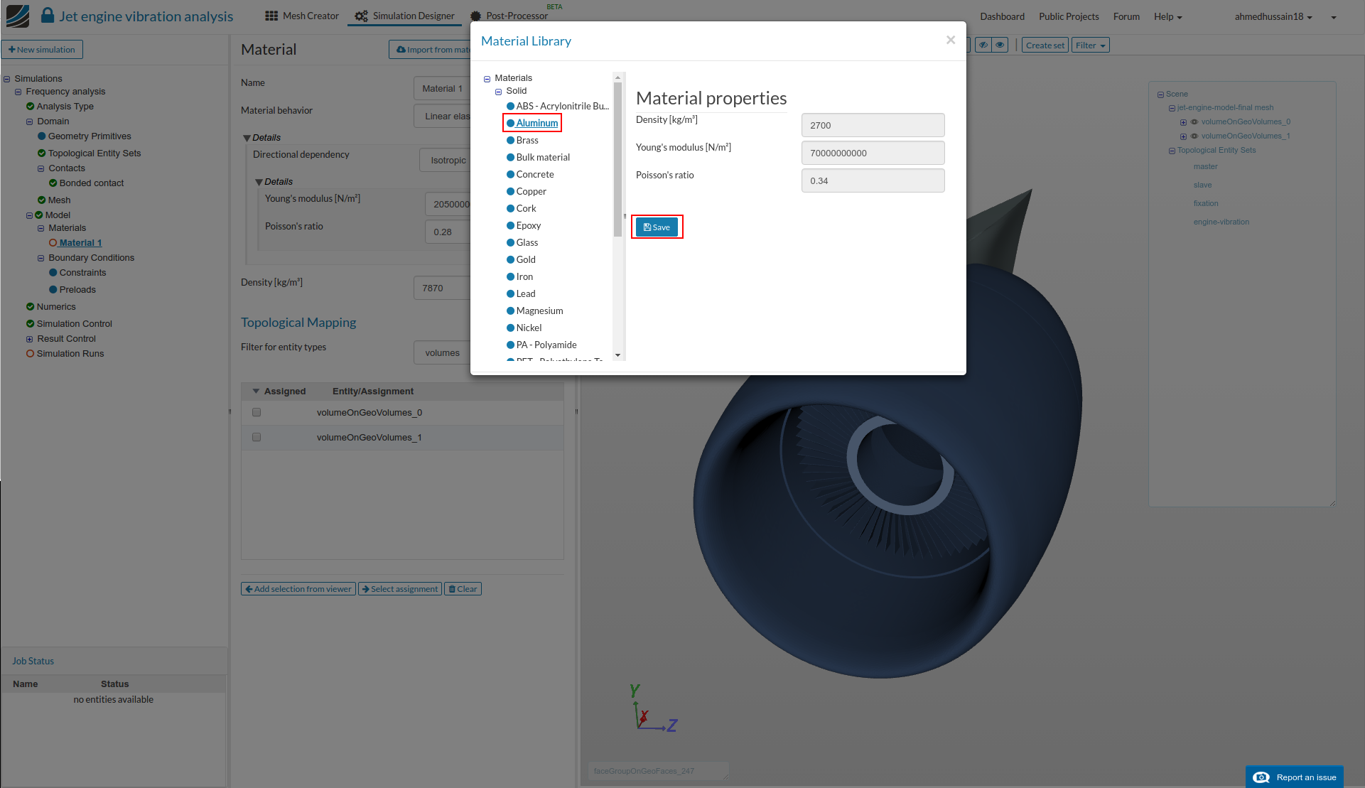
- Select ‘Aluminum’ from the material library database and click ‘Save’ to import the material in to the simulation setup.
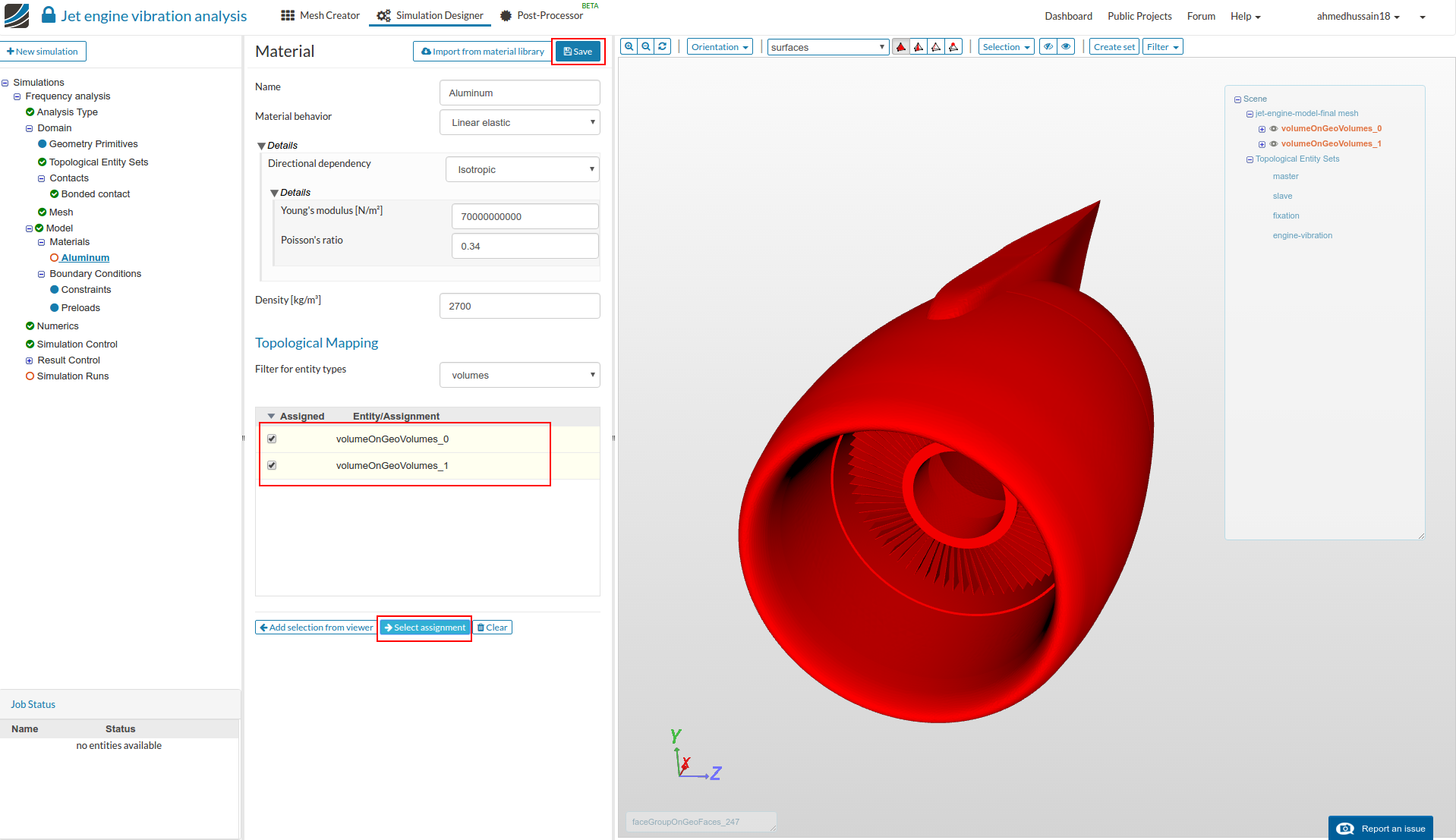
- Select both volumes under ‘Topological Mapping’ and click ‘Select assignment’ to see the selected assignment highlighted in the viewer. Click ‘Save’ to register the material definition.
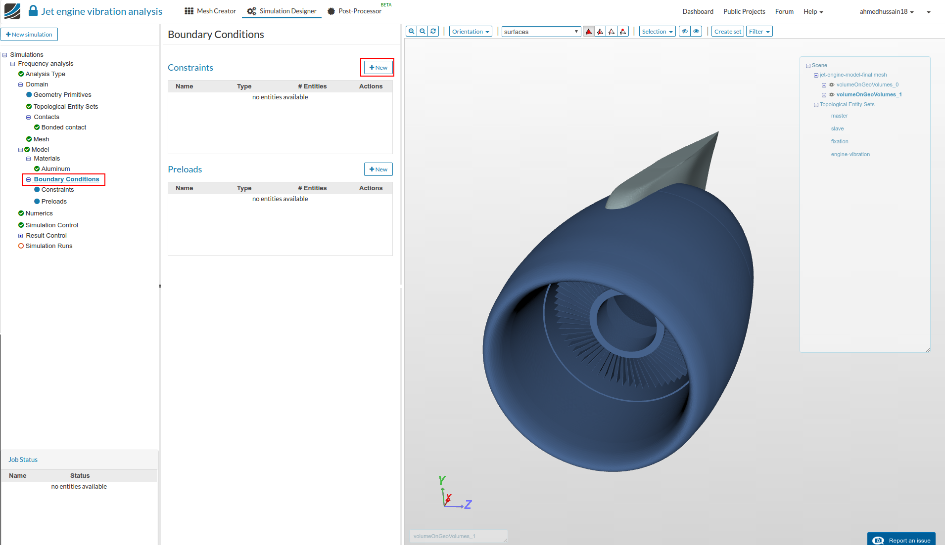
Boundary Conditions
-
For the frequency analysis in order to just get the natural frequencies of the cowling mounted on the wing via pylon, we only need to define the fixation of it with the wing.
-
Go to ‘Boundary Conditions’ under simulation tree and click ‘New’ next to constraint to define the fixation boundary conditions.
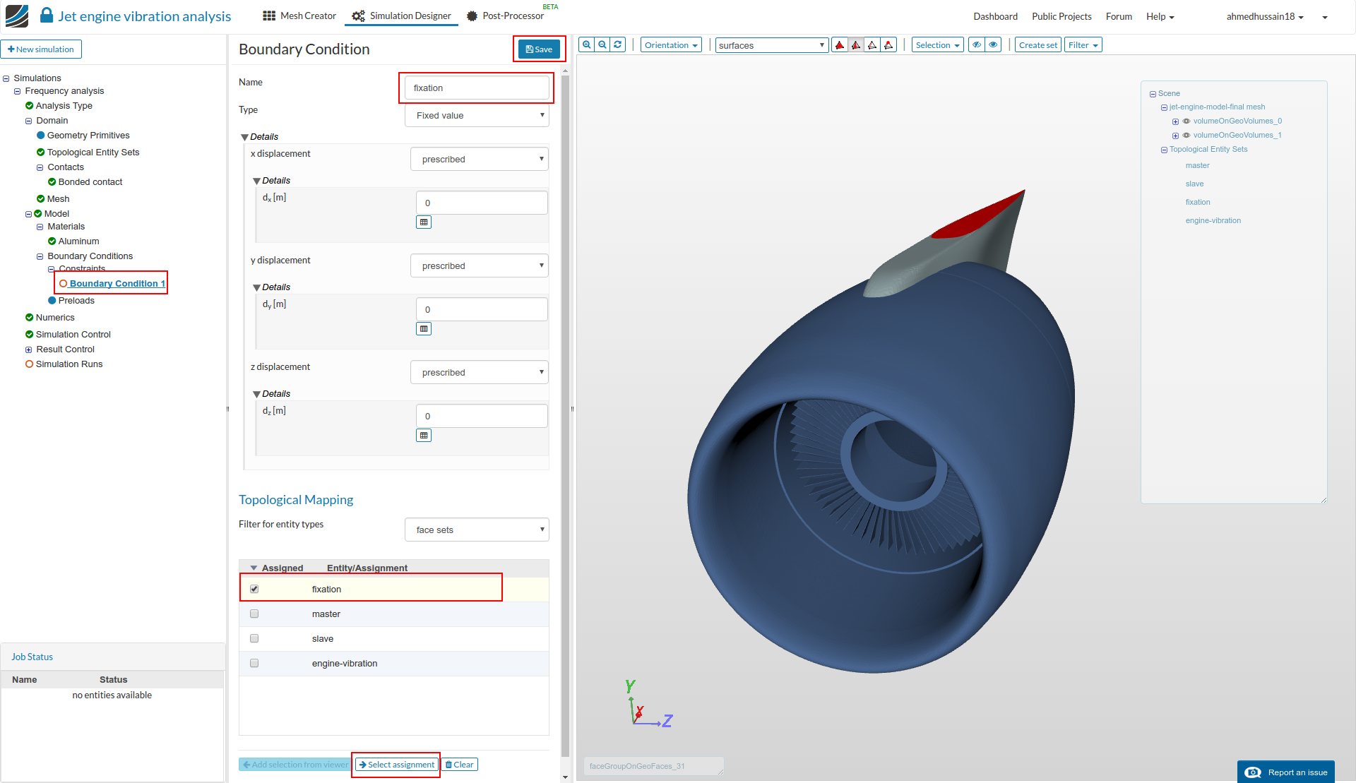
- Give newly created boundary condition a reasonable name e.g. fixation in this case and then select ‘fixation’ under ‘Topological Mapping’. Click ‘Select assignment’ to see the selected entity highlighted in the viewer. Click ‘Save’ to register changes.
Simulation Control
- Click on ‘Simulation control’ and change ‘Number of computing cores’ to 8. Change ‘Number of eigenfrequecies [-]’ to 20 and then click ‘Save’ to register the changes.

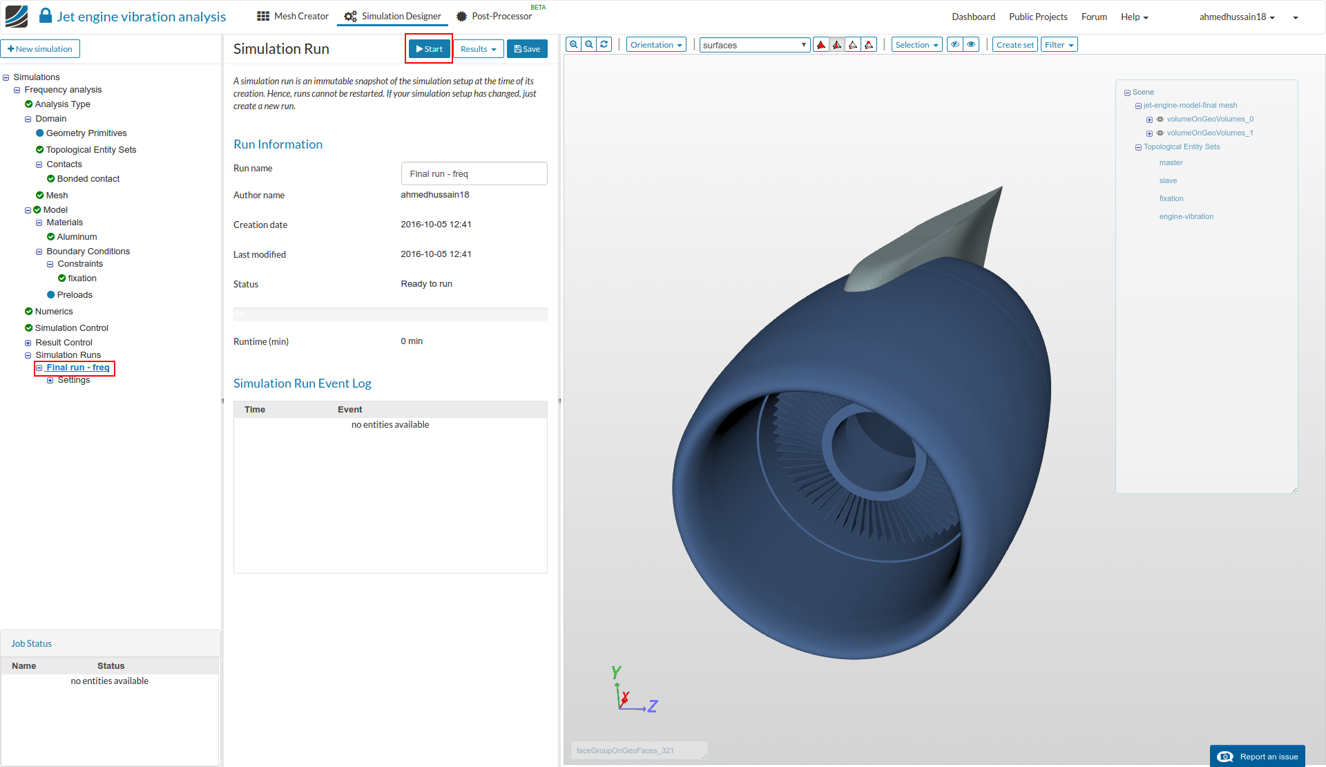
Simulation Run
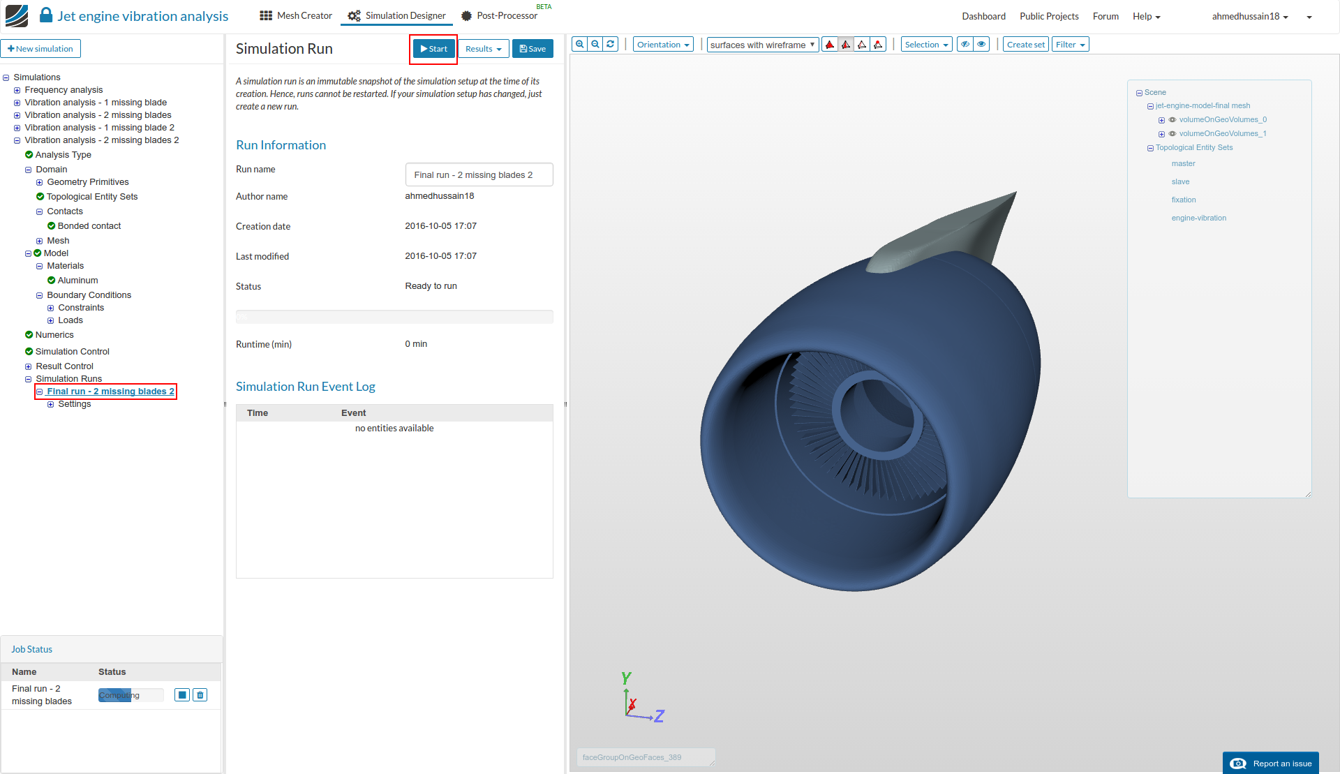
- All good for creating our frequency analysis simulation run. Go to Simulation runs and create a ‘New’ run. Give simulation run a suitable name in the pop-up window that appears e.g. Final run - freq (optional) in this case. Click ‘Create’ to create a new run. (Ignore the warnings that pops-up)

- The new run will be created under ‘Simulation Runs’. Click ‘Start’ to run the simulation.
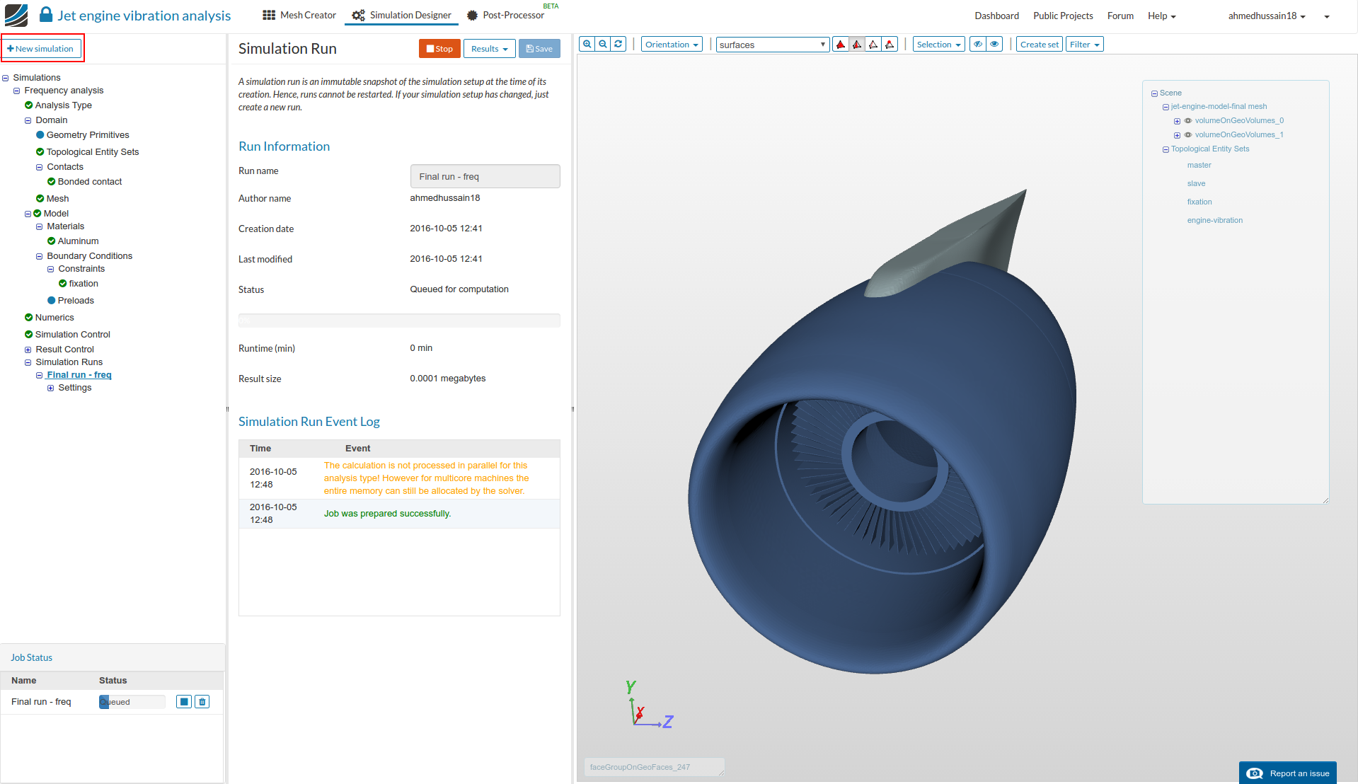
-
The simulation run will take approx. 15 min. to finish.
-
Before you create the simulation run for further configurations, it is recommended to let this simulation complete so that you can review the results of it since these results are prerequisite for the harmonic analysis case. You can proceed directly from here to ‘Post-processing’ of ‘Configuration 1’ in order to see the modes we are interested in.
Create Further Configurations
Configuration 2:
- While the frequency analysis run is under computation, go ahead and make a new simulation in order to perform the harmonic analysis considering missing blade vibration load.
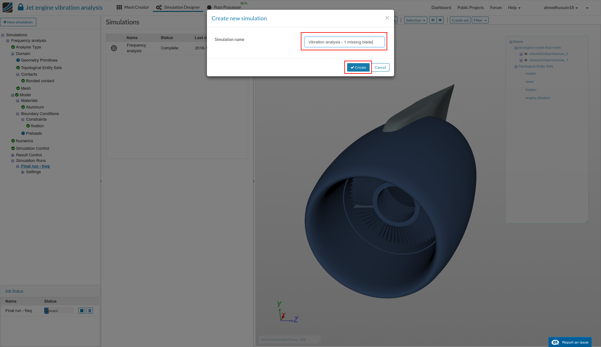
- Name the simulation Vibration analysis - 1 missing blade and click ‘Create’ in order to create new simulation.
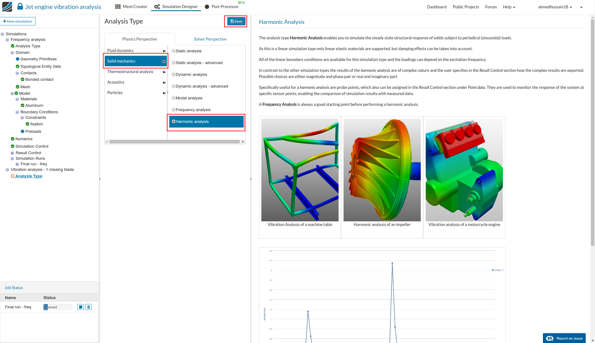
- Select ‘Harmonic analysis’ under ‘Solid mechanics’ as analysis type and click ‘Save’ to register changes.
-
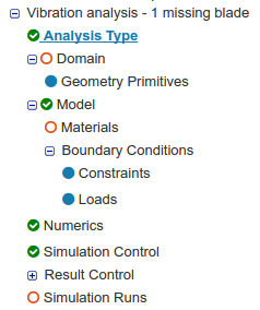
The simulation tree will look something like this:
-
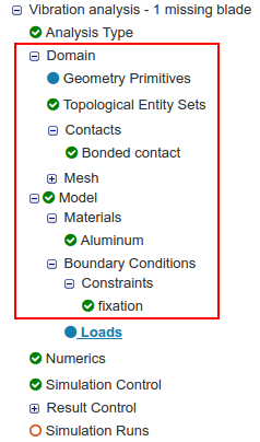
Now follow all the above steps of ‘Configuration 1’ until ‘Boundary Conditions’. At the end your simulation tree should look something like this:
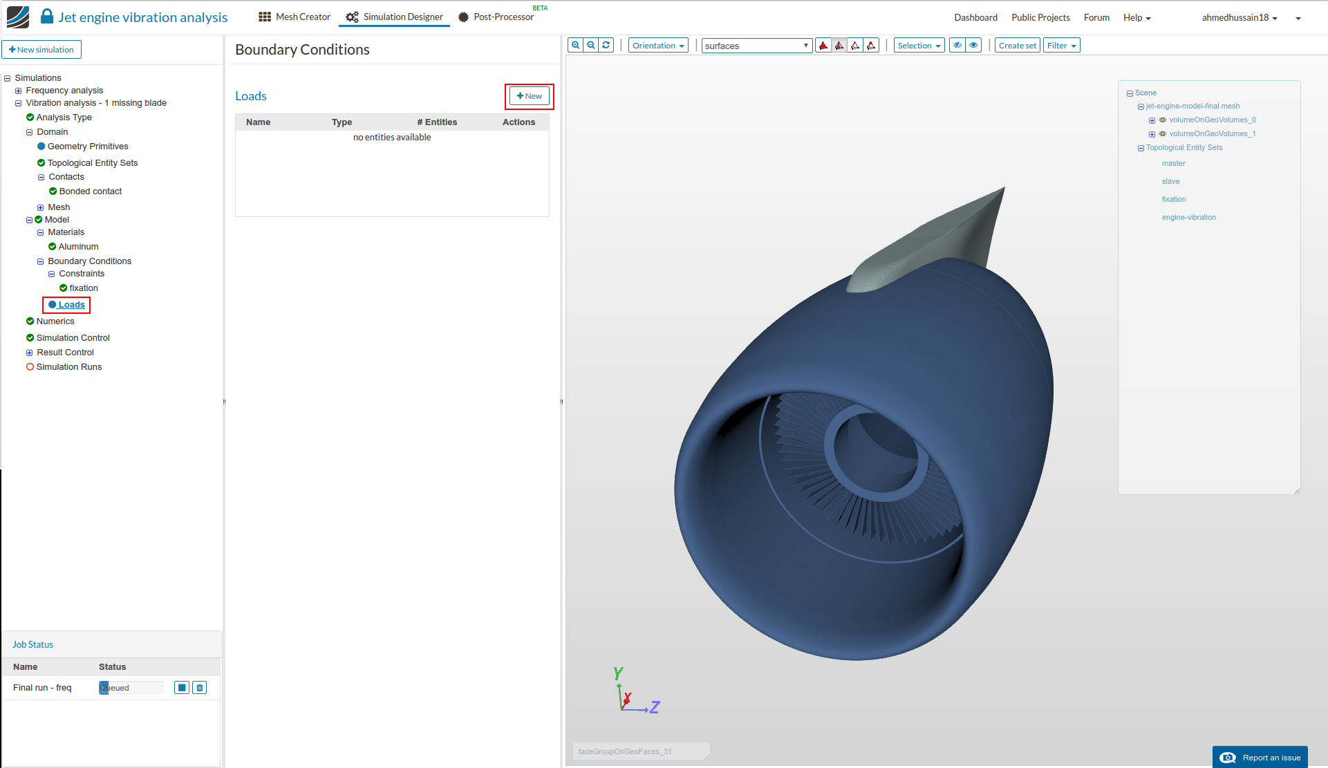
Loads:
-
After setting up the simulation until ‘Constraint’, we will now define the loads to the internal surfaces of the cowling on which the jet engine is connected. The applied force load is calculated considering the following formulaton:
<img src="/forum/uploads/default/original/2X/2/20c8606f605b4d9de1d4382a5168dfa811fe1511.png" width="678" height="239"> -
We will consider that our fan blade is made of titanium. Considering the density of the titanium as equivalent to 4500 kg/m3, the mass of a missing blade is found out to be ~7.65 kg. The distance of the dislocated center of mass is found out to be 5e-3 m. We will consider the load only in y and z direction since the rotational axis of the jet engine blade is x axis.
Jet engine load - Fy:
- Go to ‘Load’ under simulation tree and click on ‘New’ to create a new load.
-
Rename newly created load to Jet engine load - Fy, change ‘Type’ to Force, change value of ‘fy [N]’ to 1.
-
Next click on ‘f(x)’ and give this in the formula tab: _7.65(5e-3)4(pi^2)*(f^2)_*
-
Select ‘engine-vibration’ under ‘Topological Mapping’, click ‘Select assignment’ to see the selected assignment highlighted in the viewer. Click ‘Save’ to save the first load case.

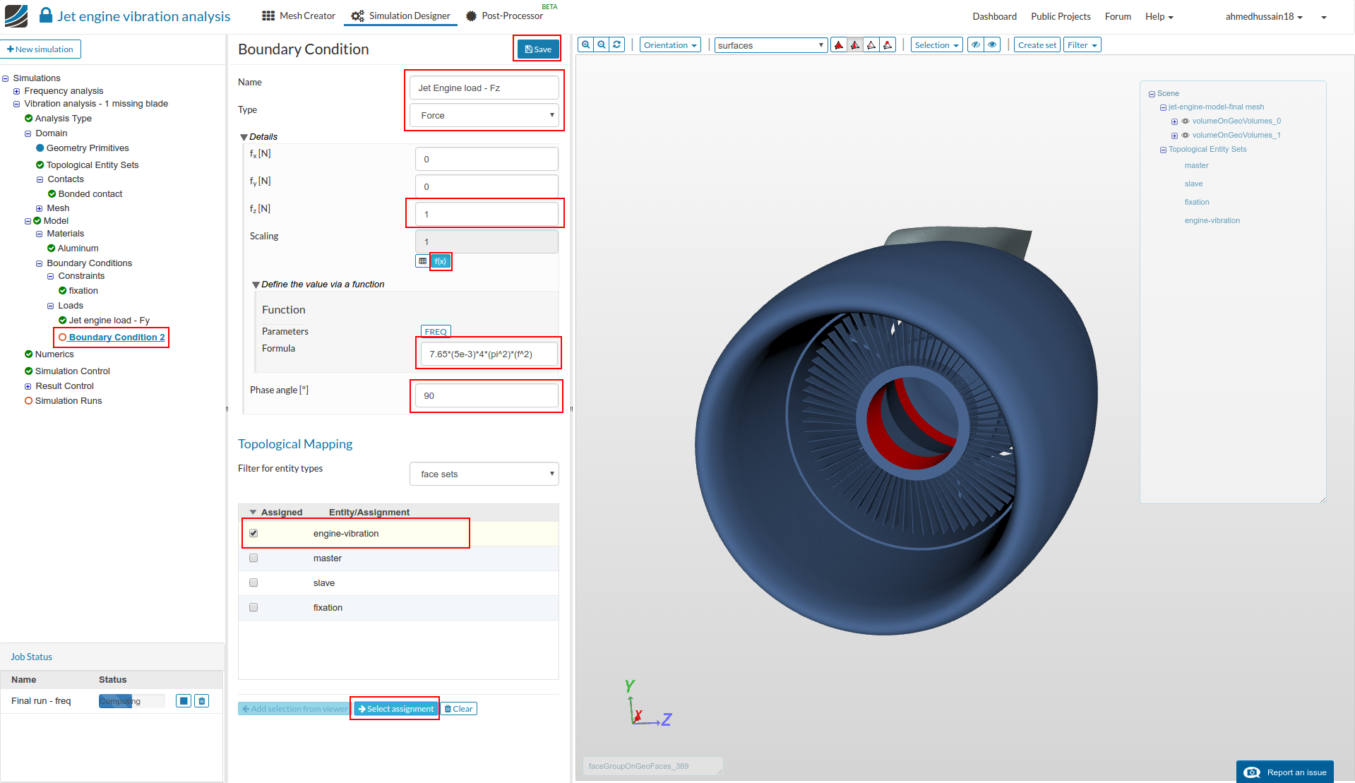
Jet engine load - Fz:
- Follow the same procedure as above but this time rename the load to ‘Jet engine load - Fz’, give value of 1 next to ‘fz [N]’ instead of ‘fy [N]’, give the same formula under ‘f(x)’ and give value of 90 next to ‘Phase angle [°]’. Click ‘Save’ to register your changes for the second load.
Numerics
- Go to ‘Numerics’ and change ‘Equation solver’ to MUMPS. Click ‘Save’ to register changes.
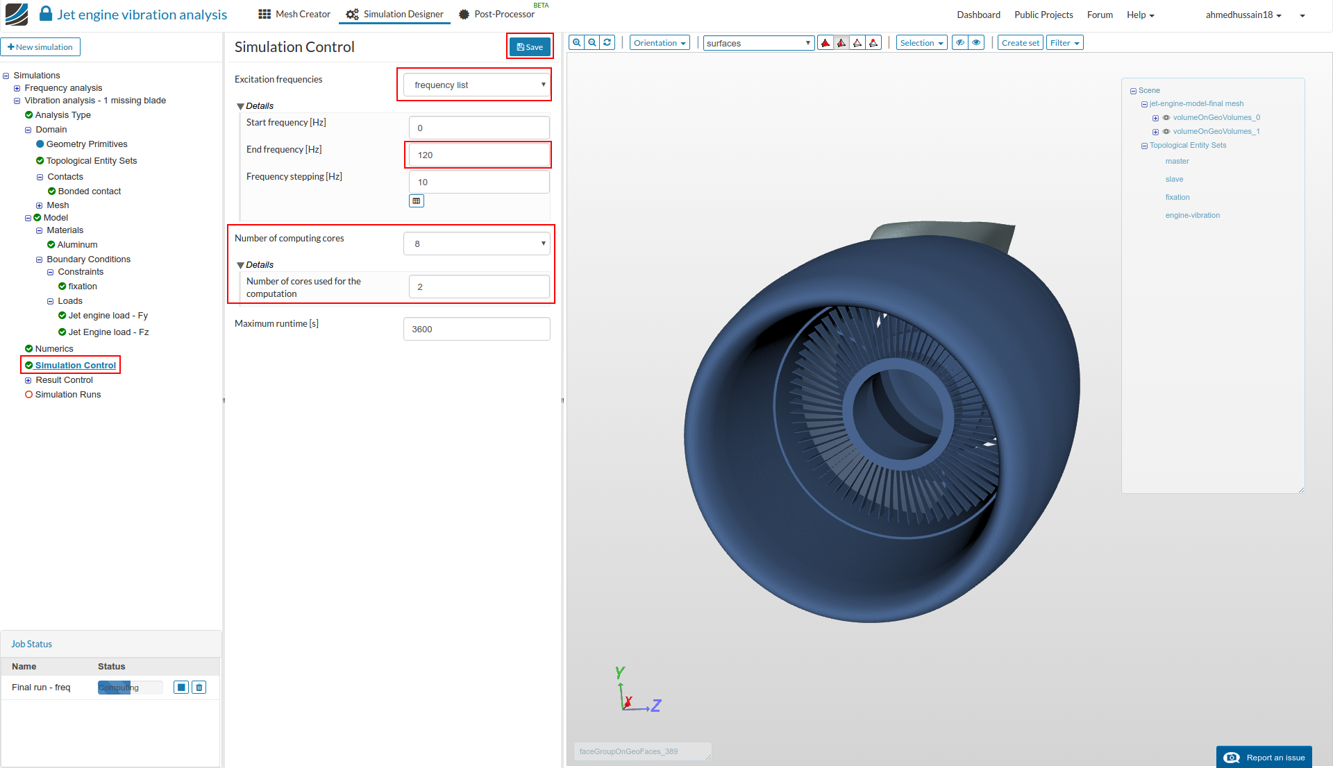
Simulation Control
- Go to ‘Simulation Control’ and change ‘Excitation frequencies’ to frequency list, change ‘End frequency [Hz]’ to 120 (which is our interesting range since jet engines normally run between 3000 (50 Hz) to 6000 rpm (100 Hz)),‘Number of computing cores’ to 8 ‘Number of cores used for the computation’ to 2. Click ‘Save’ to register changes.
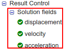
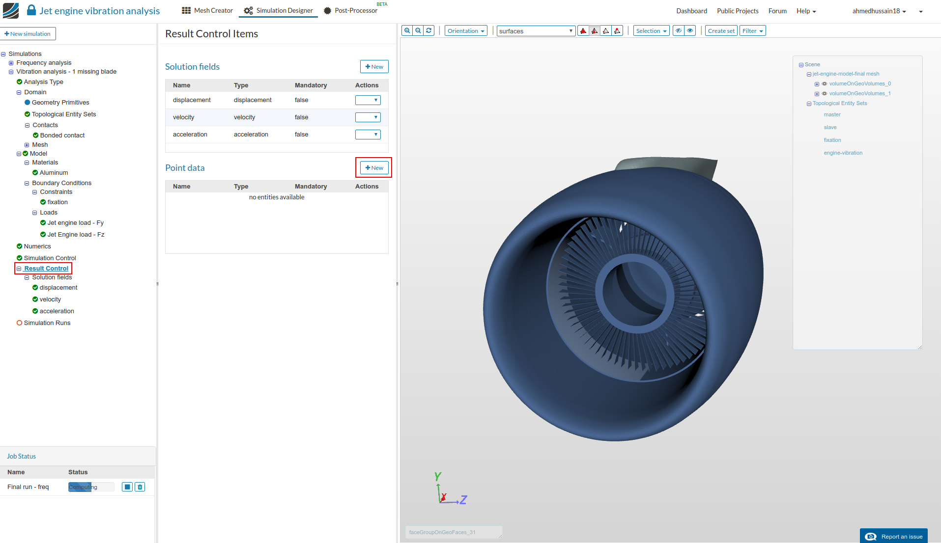
Result Control
-
Go to ‘Solution fields’ under ‘Result Control’ and delete ‘cauchy stress’ and ‘total strain’ as we are not interested in these quantities, thus deleting it will save some computation time.
-
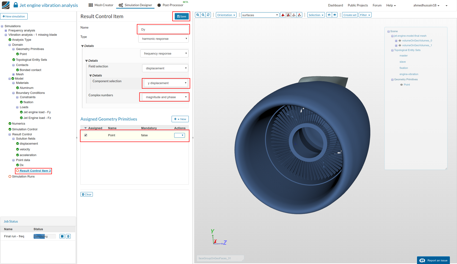
Next click ‘Result Control’ in simulation tree and click ‘New’ in front of ‘Point’ to create a new point calculation method which will plot the magnitude and phase of displacement on a specific point.
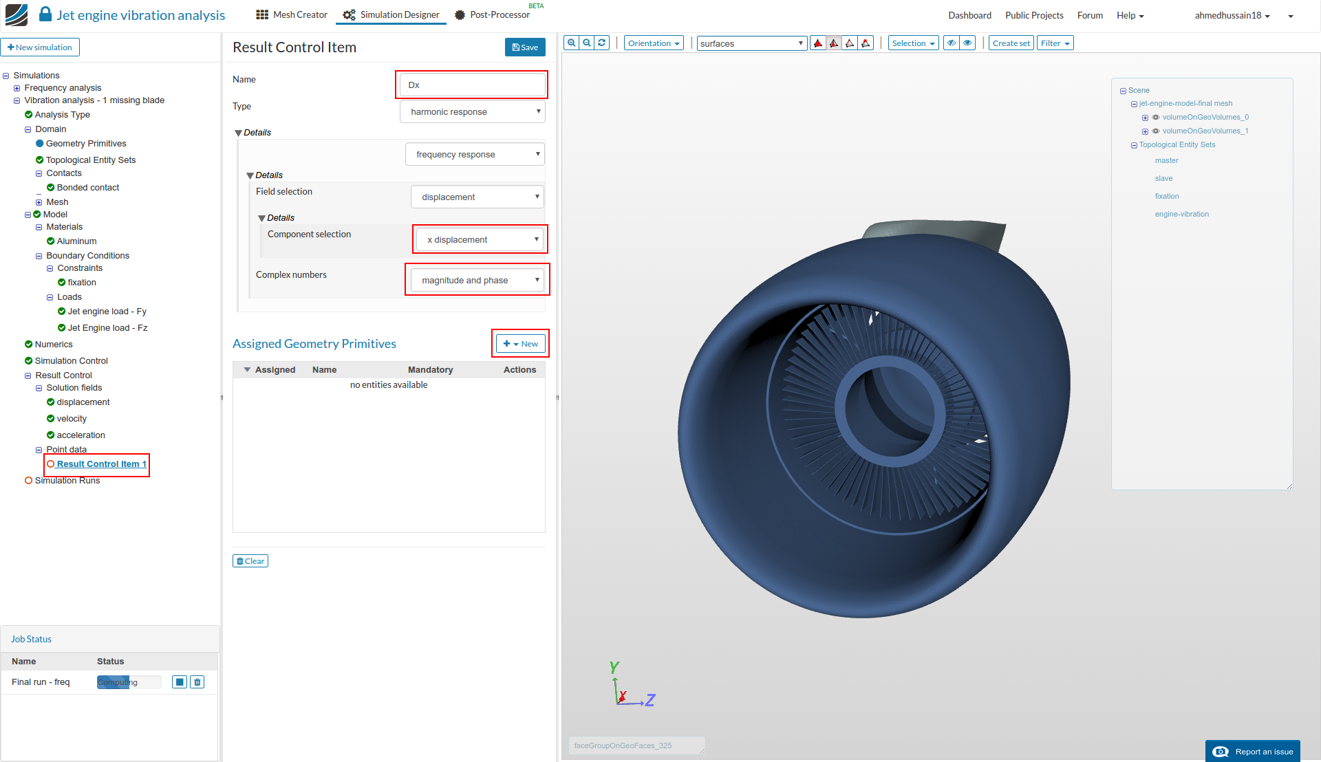
- Rename it to ‘Dx’ (optional), change ‘Component selection’ to x displacement and ‘Complex numbers’ to magnitude and phase. For this calculation method next we need a point along which the displacement graph will be plotted. For this click ‘New’ next to ‘Assigned Geometry Primitives’ and click on ‘Point’. This operation will require you to save changes for the current point calculation definition. Therefore save it for later use.
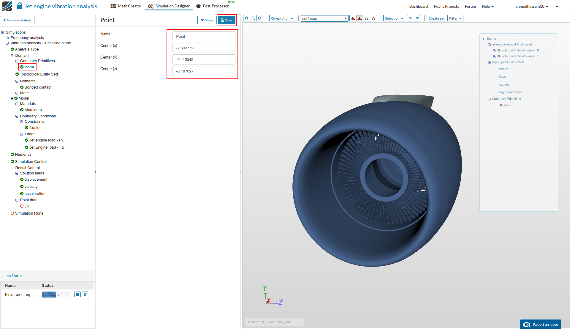
- Under ‘Geometry Primitives’, give following values as x,y and z coordinates of your point: -2.333779, -0.115045 and -0.407097. Click ‘Save’ to save the point. You will now see a point in inner circular area of stator.
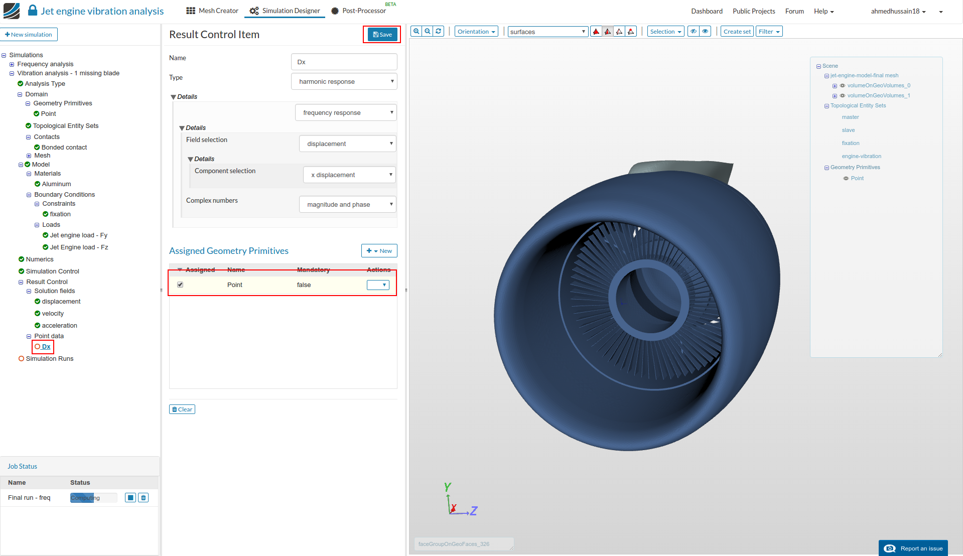
- Next go back to ‘Dx’ point calculation definition and select the created point under ‘Assigned Geometry Primitives’ and click ‘Save’ to save changes.
- Similarly, perform the same steps to create the point calculation method for y and z displacements. This time you don’t have to create a new point as it has already been defined.

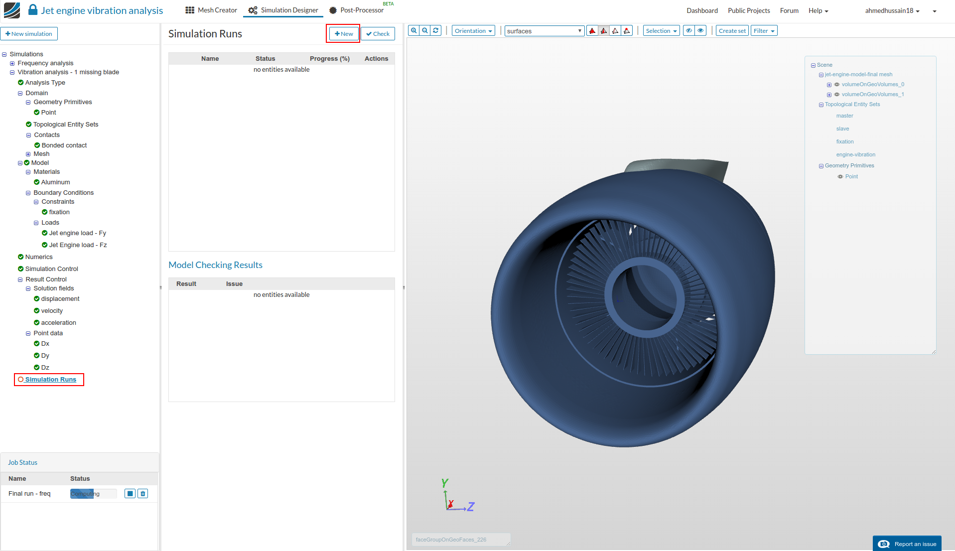
Simulation run
- That’s it for the ‘Configuration 2’. Create a new simulation run under ‘Simulation Runs’ and rename it to ‘Final run - 1 missing blade’ (optional) and click ‘Start’ to start the run.

- Simulation run will take approx. 30 min. to finish.
Configuration 3
-
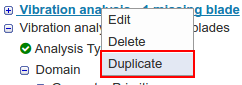
While ‘Configuration 2’ simulation run is in computation phase, go ahead and duplicate the ‘Configuration 2’ simulation i.e. Vibration analysis - 1 missing blade in this case.
<img src="/forum/uploads/default/original/2X/7/709bed3afa2e30e85ada6dcd1bb2012d3ff63a57.png" width="251" height="83"> -
Rename it to Vibration analysis - 2 missing blades and click ‘Save’.
-
Since we are looking forward to simulate the vibration impact of the jet engine missing 2 fan blades, all we have to do is to change our loads.
-
Go to ‘Jet engine load - Fy’ and change ‘Formula’ to: _15.3(8.42e-3)4(pi^2)*(f^2)_*. Click ‘Save’ to register your changes.
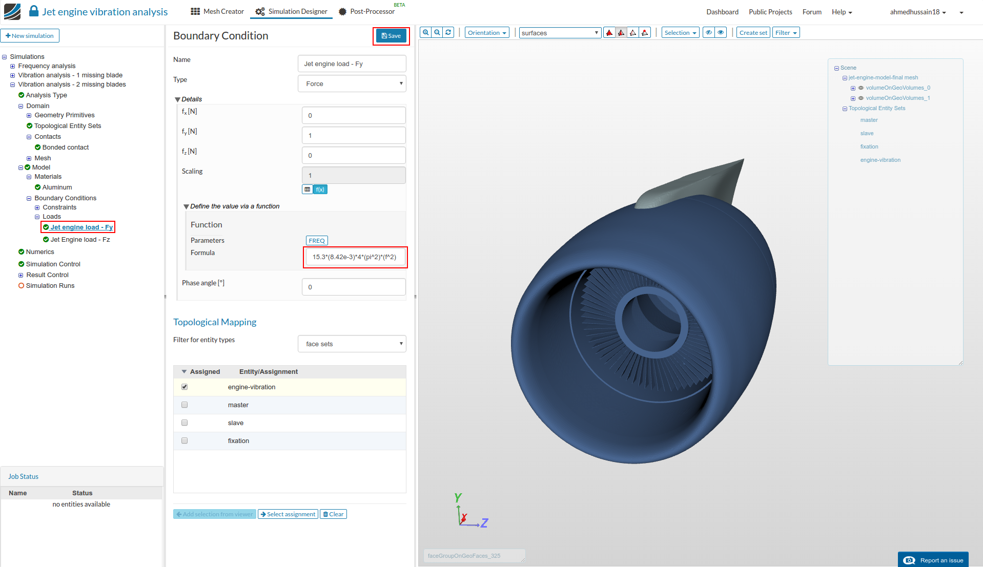
- Similarly, do the same for ‘Jet engine load - Fz’. Click ‘Save’ to register your changes.

- Next create a new run under ‘Simulation Runs’. Rename the run to ‘Final run - 2 missing blades’. Click ‘Start’ to start the run.
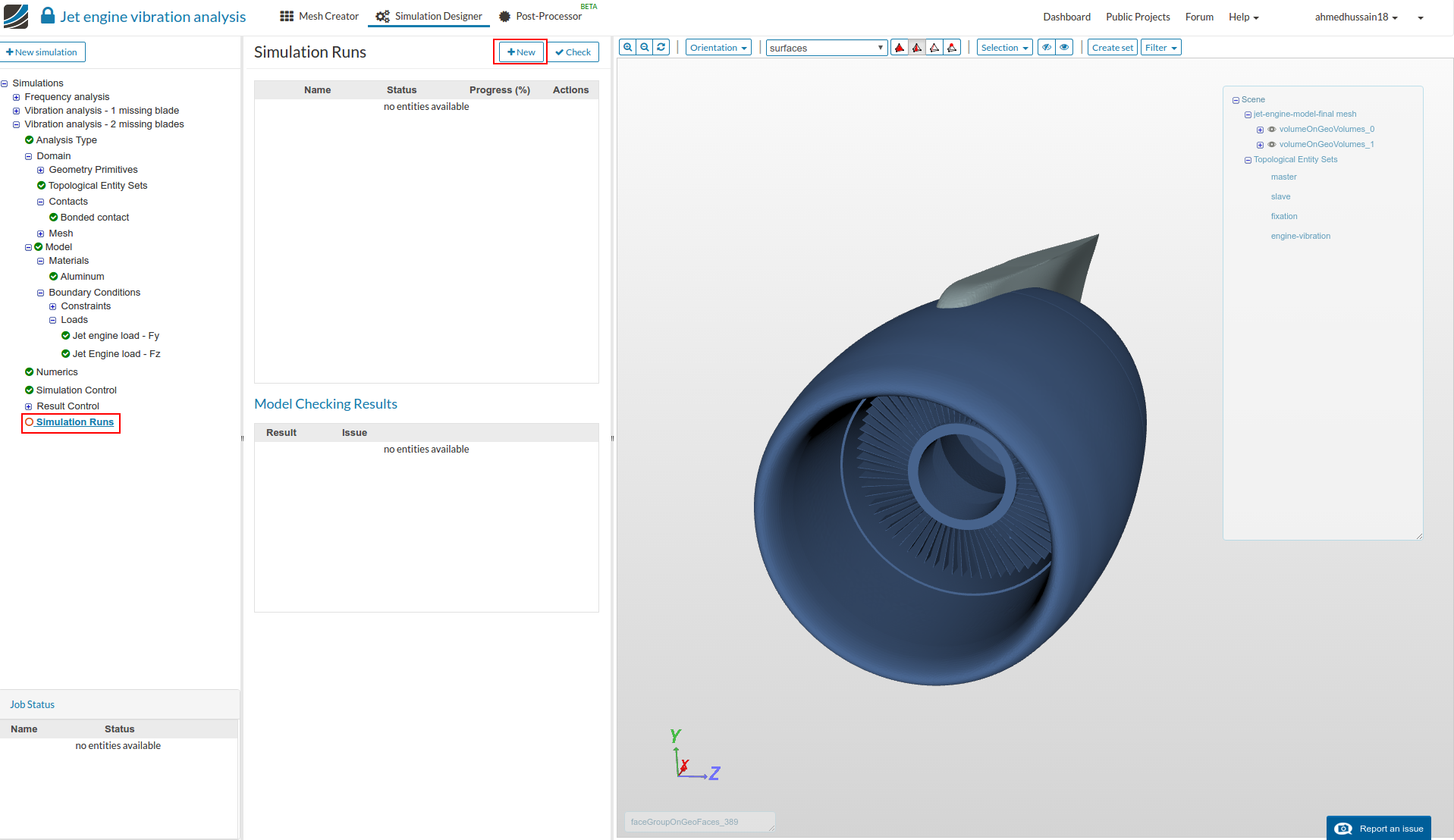

-
Simulation run will take approx. 30 min. to finish.
-
Before moving to the next configurations it is recommended to let ‘Configuration 2’ and ‘Configuration 3’ to complete. Based on there results the trimmed frequency range for the next configurations is decided. For better understanding, let these simulations complete and then move to the ‘Post-processing’ section to have better understanding before setting up the next configuration cases.
Configuration 4
-
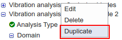
For ‘Configuration 4’, duplicate ‘Configuration 2’ i.e. Vibration analysis - 1 missing blade.
-
Based on the results from ‘Configuration 2’, it is evident that the peak of displacement is between 80 to 120 Hz. Therefore, we will now redefine our frequency range and rerun the case in order to get the exact frequency where the peak displacement is taking place.
-
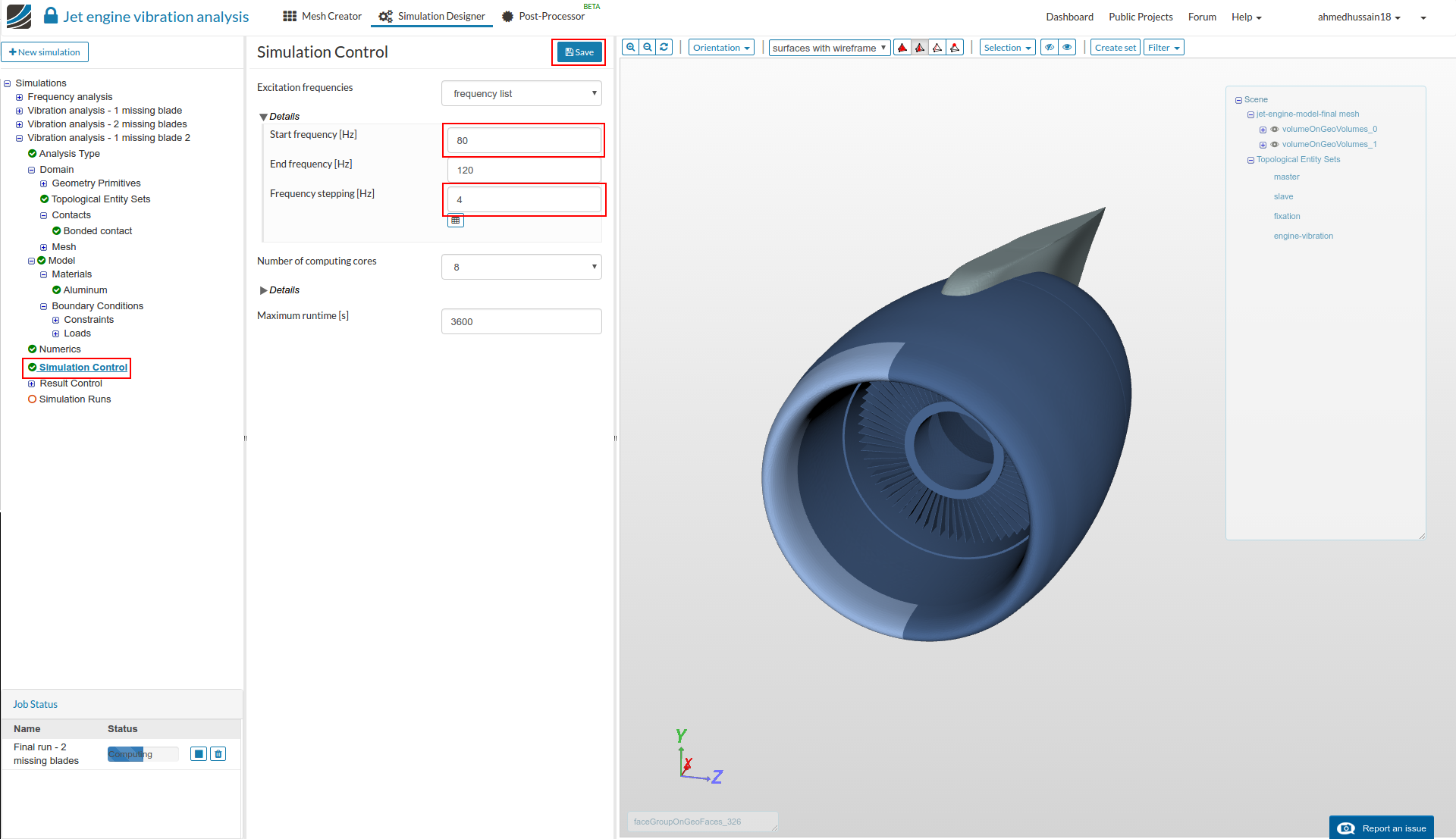
Go to ‘Simulation Control’ and change ‘Start frequency [Hz]’ to 80 and ‘Frequency stepping [Hz]’ to 4. Click ‘Save’ to register changes.
- Next go to ‘Simulation Runs’, create a new run and rename it to Final run - 1 missing blade 2, click ‘Start’ to initiate the run.
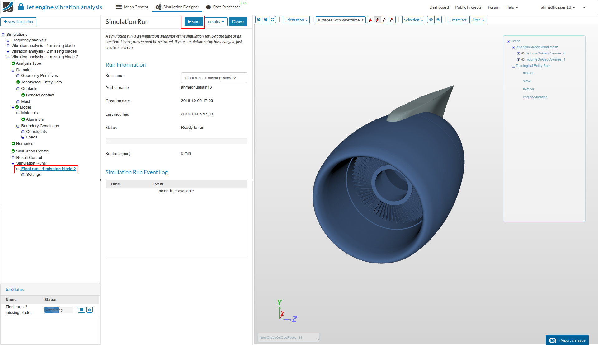
- Simulation run will take approx. 30 min. to finish.
Configuration 5
- For ‘Configuration 5’, duplicate ‘Configuration 3’ i.e. Vibration analysis - 2 missing blades.
-
Based on the results from ‘Configuration 3’, it is evident that the peak of displacement is between 80 to 120 Hz. The only difference compared to ‘Configuration 2’ is that the peak is bit higher. Therefore, we will now redefine our frequency range and rerun the case in order to get the exact frequency where the peak displacement is taking place.
-
Go to ‘Simulation Control’ and change ‘Start frequency [Hz]’ to 80 and ‘Frequency stepping [Hz]’ to 4. Click ‘Save’ to register changes.

- Next go to ‘Simulation Runs’, create a new run and rename it to Final run - 1 missing blade 2, click ‘Start’ to initiate the run.
- Simulation run will take approx. 30 min. to finish.
Post-processing
Frequency analysis (Configuration 1):
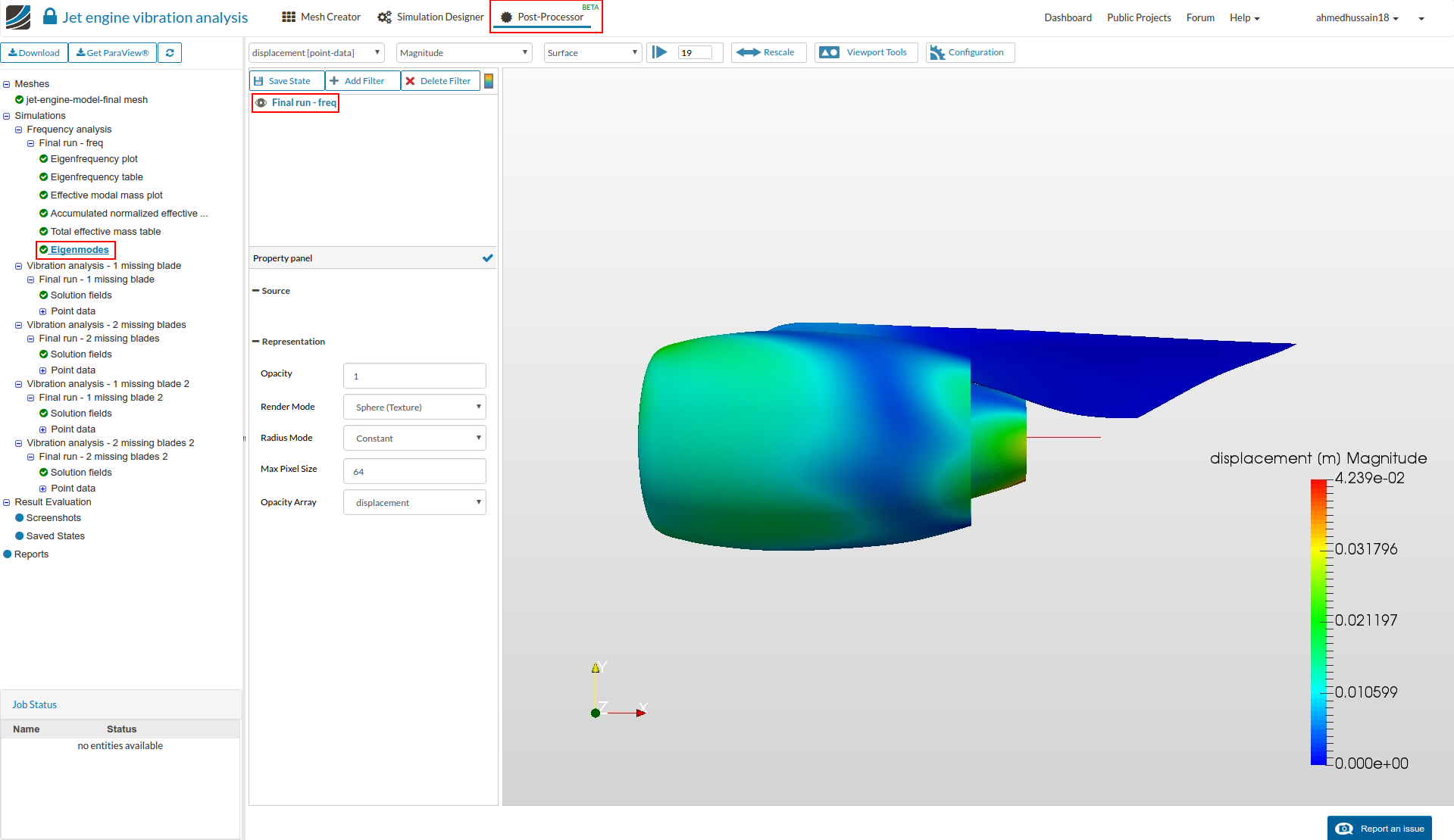
- Once the simulation run of Configuration 1 is finished. Go to the ‘Post-Processor’ and click on ‘Eigenmodes’. After a while the solution will be loaded in the viewer.
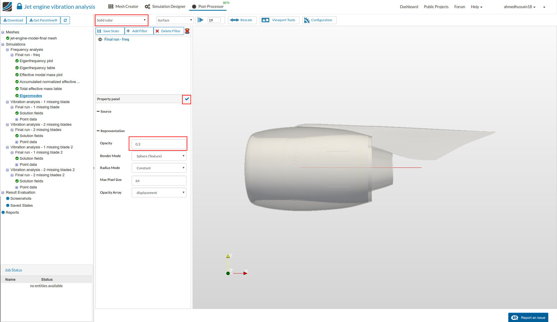
- Change ‘Aray name’ to ‘Solid color’ from top and then ‘Opacity’ under representation to 0.3. Click blue tick to save the settings. This will make model transparent.
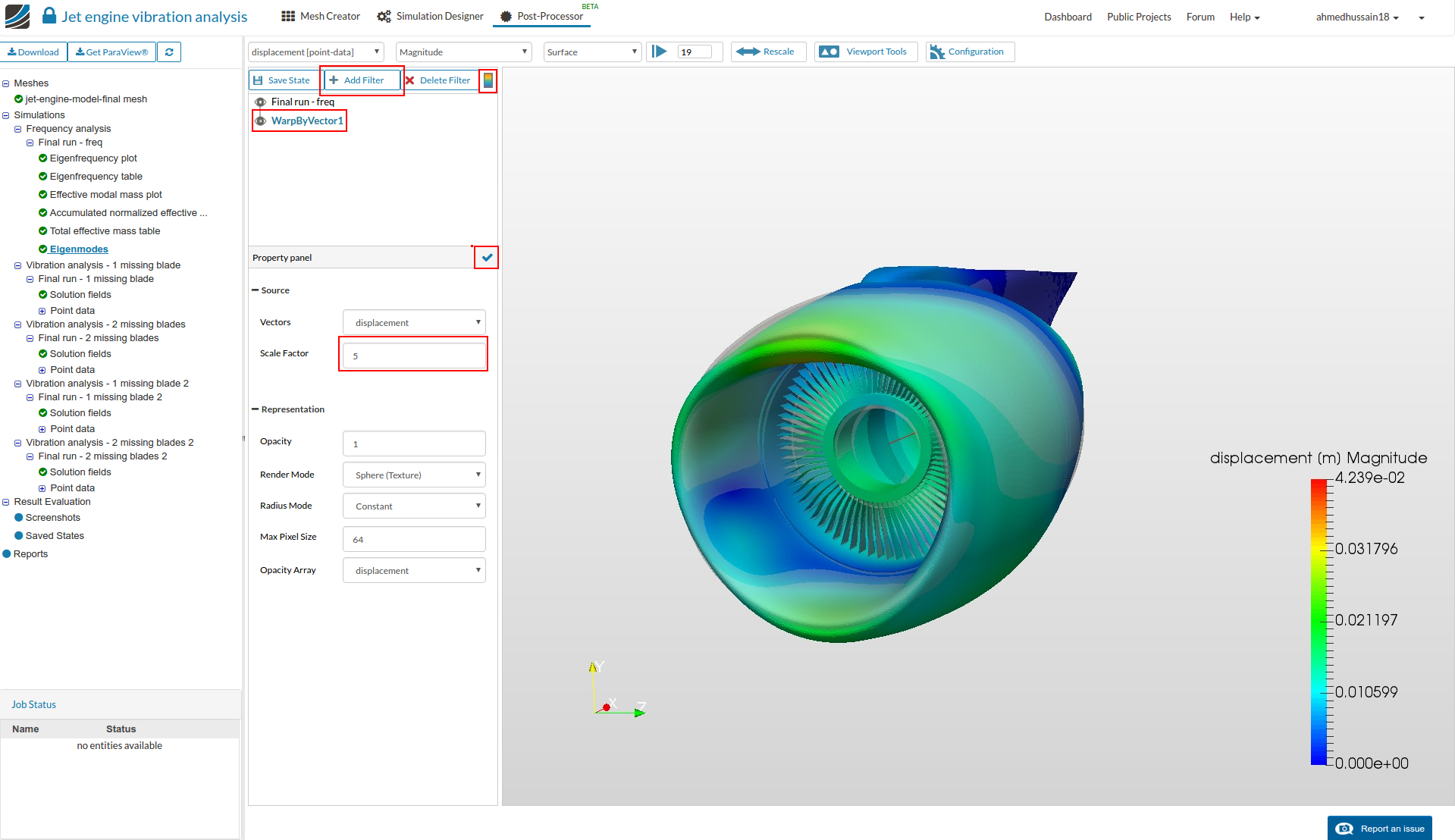
- Next, add a ‘WarpByVector’ filter by clicking on ‘Add filter’ button in the middle top. Change ‘Scale Factor’ to 5 in order to scale the displacement 5 times. Click blue tick button to save changes.
- Click ‘Play’ in timestep window to see all the eigenmodes. It is evident that the first 10 eigenmodes are the one which produces the vibration which are interesting in our case. Other than that we can ignore the rest eigenmodes.

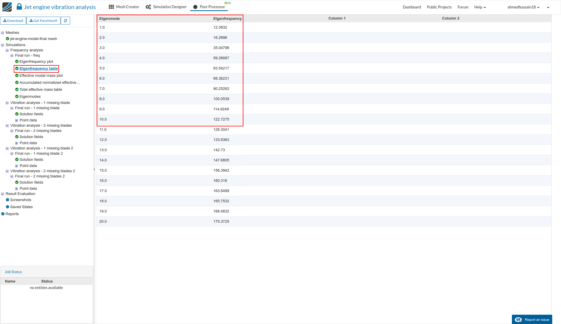
- You can also click on ‘Eigenfrequency plot’ to see the plot of frequencies.

- Whereas the ‘Eigenfrequency table’ is a good way to see the table of eigenmodes and their corresponding eigenfrequencies. We can see that the first 10 frequencies are under 0 10 130 Hz range.
- The animation of the modes is shown below (This animation is made using local Paraview):
Harmonic analysis (Configuration 2 & 3):
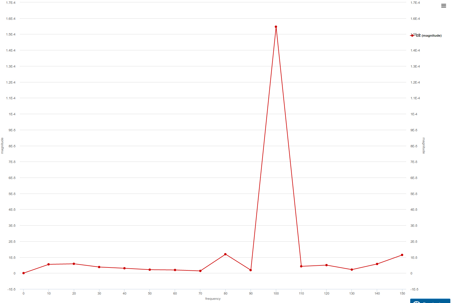
- Based on the frequency analysis result, the vibration was studied for the missing blade vibration load with in the frequency range of 0 to 120 Hz (rotational speed of 0 to 7200 rpm). The most important result in this case is the displacement plot in y and z direction. Below are the displacement plots of ‘Configuration 2’:

and that of ‘Configuration 3’:
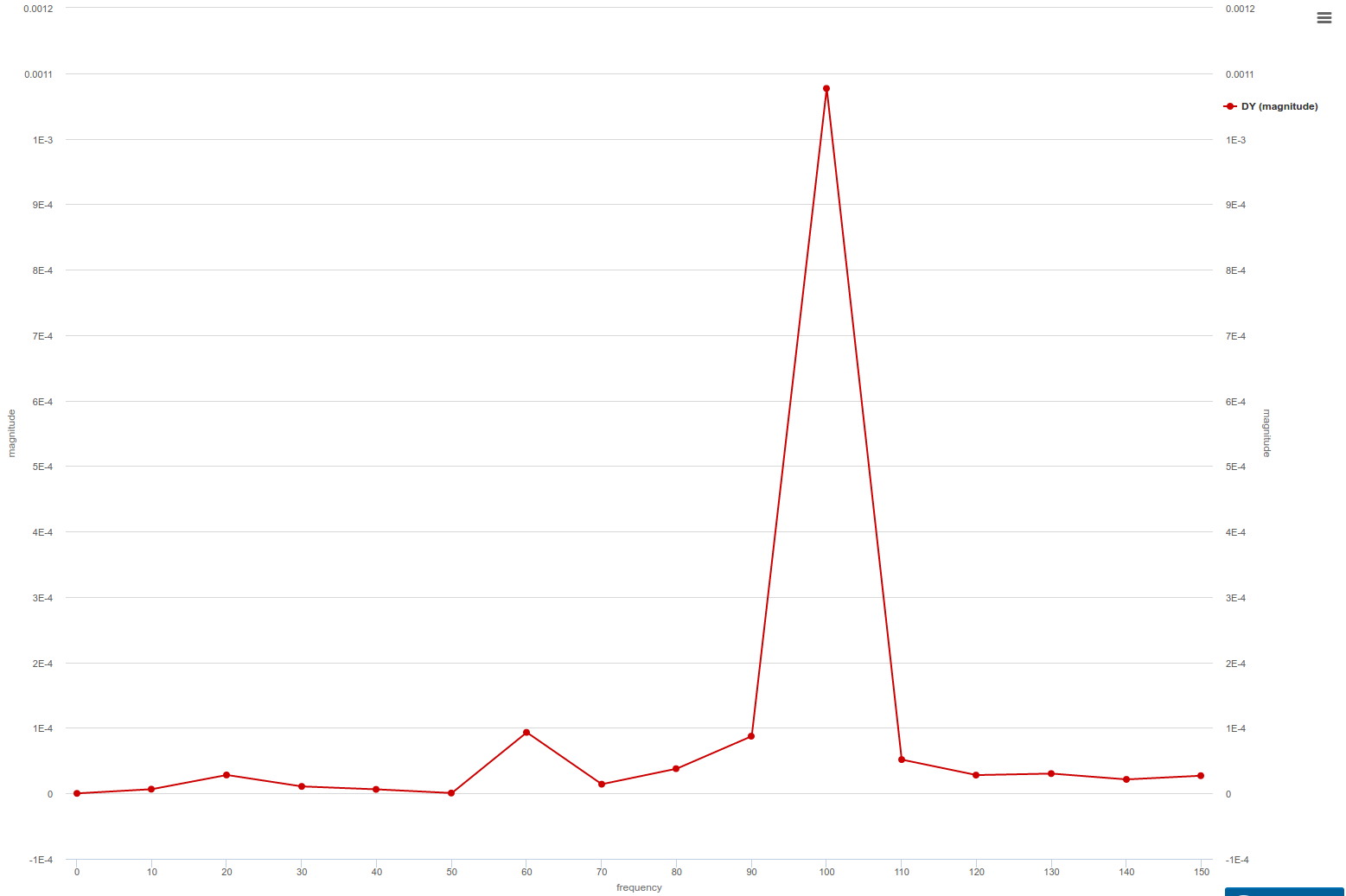
- It can be seen that the only difference between two configurations i.e. simulation with 1 and 2 missing blades is the magnitude of displacement. In case of 2 blades, only the magnitude is higher. Thus the most interesting thing in this case is that is the peak of the displacement between 100 and 110 Hz. This peak is showing that at around this frequency the cowling will vibrate the most. But these results are based on a coarse measurement, therefore we will create ‘Configuration 4’ and ‘Configuration 5’ in order to focus on a refined frequency range. Looking from the above graphs, 80 to 120 Hz would be a good choice.
Harmonic analysis (Configuration 4 & 5):
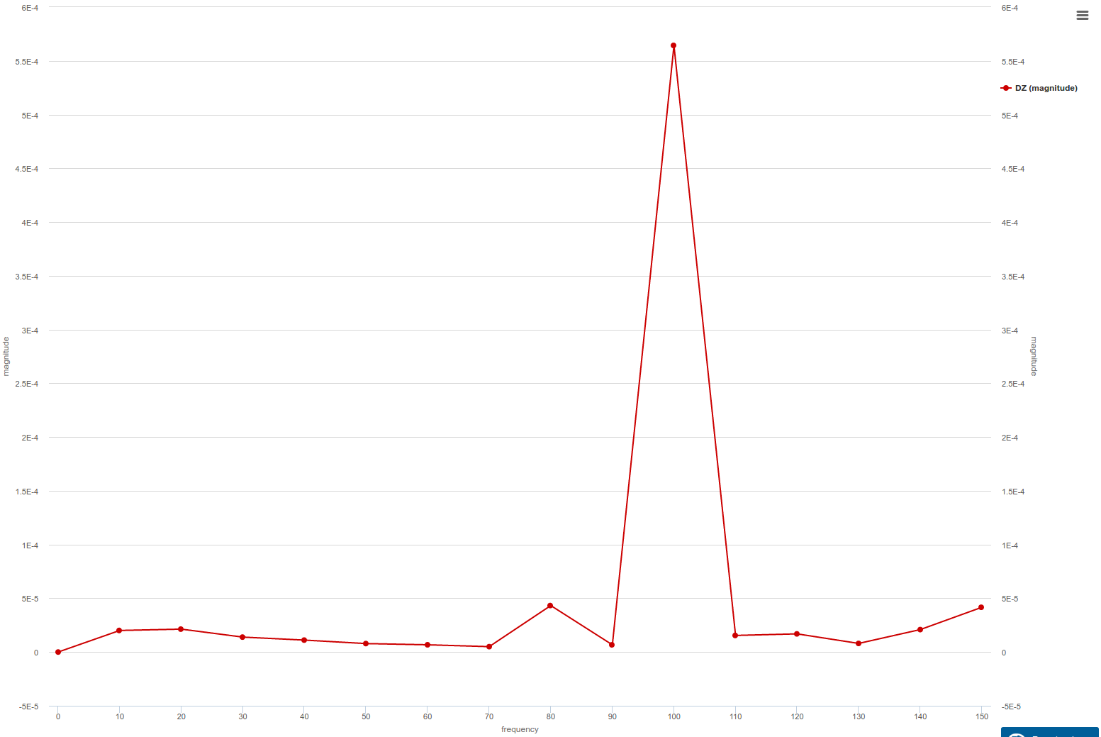
- Based on the results from Configuration 2 & 3, the same harmonic analysis with refined range of frequencies are performed. This time the graphs of ‘Configuration 4’ looks like this:

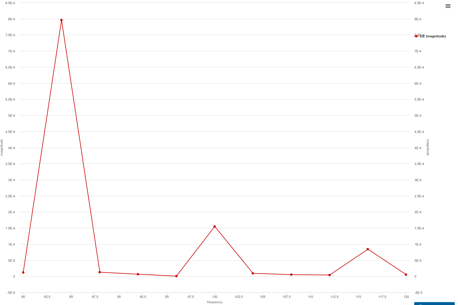
and that of ‘Configuration 5’:
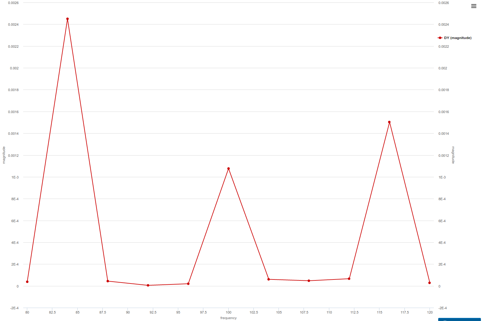
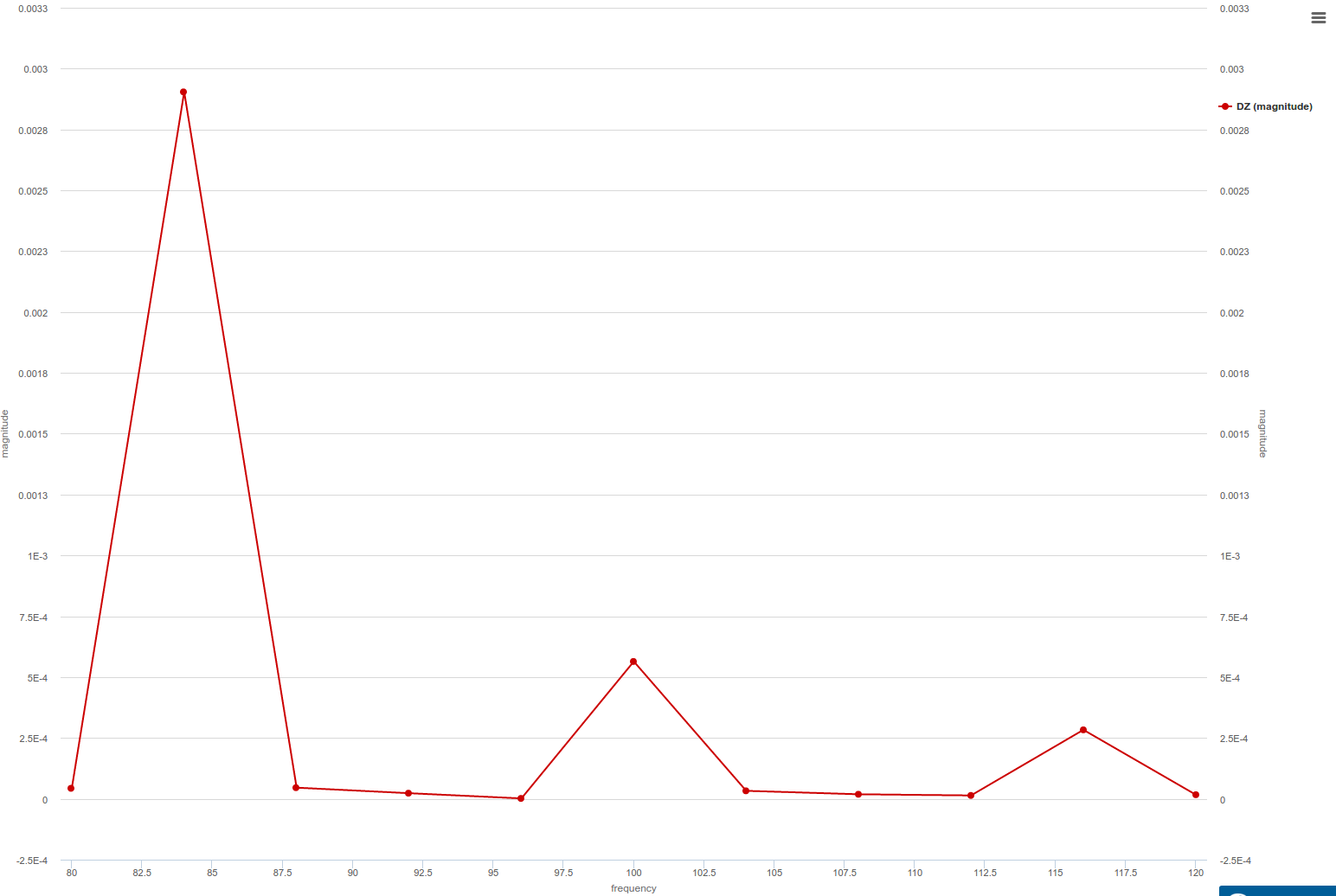
- It can be seen that now the peak occurs at 84 Hz (5040 rpm) for both cases. There are some other peaks in both cases but they are overall smaller than the one at this frequency. This shows that maximum vibration in the cowling will occur if after the loss of blade this natural frequency of the cowling is reached.

