Recording

Homework submission
Submitting all three homework assignments will qualify you for a free Professional Training (value of 500€) as well as a certificate of participation.
Homework 1 - Deadline 6th of October, 12pm
Exercise
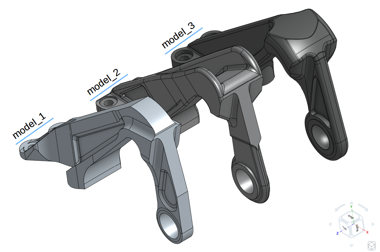
The part we are simulating in this homework is an aircraft engine bearing bracket. The function of this bracket is to support the weight of the cowling during engine service whereas it plays no active role during the operation of the engine.
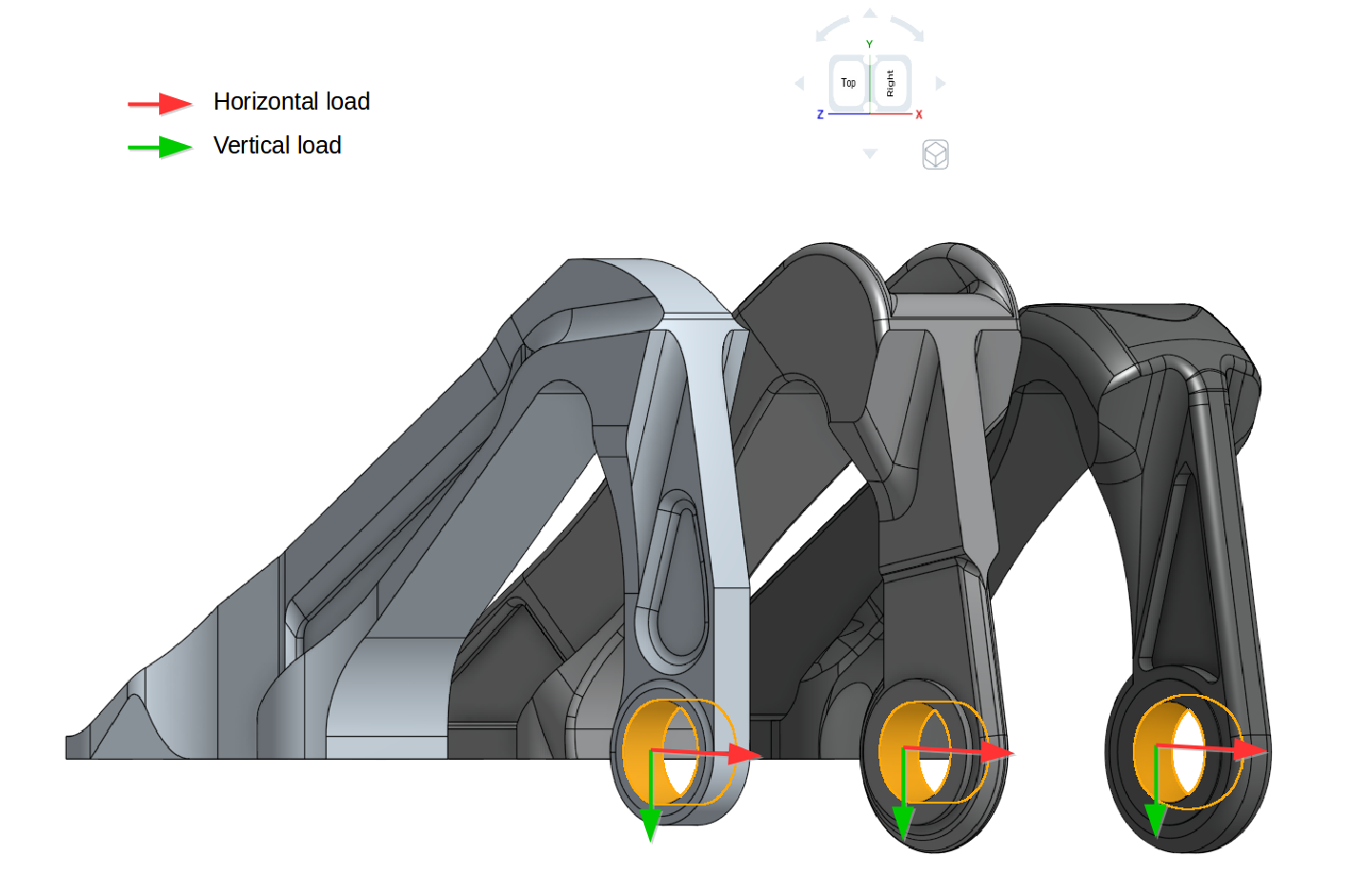
Three of the models are used in this homework provided by GrabCAD users who were the winners of the GrabCAD ‘Airplane Bearing Bracket Challenge’. The models are shown in the figure below with order of first, second and third as model_1, model_2 and model_3.
-
1st position: model_1 provided by Igor Nikolaychuk from GrabCAD. | Strength/Weight: ~99.76 kN/kg
-
2nd position: model_2 provided by Allar Õunsaar from GrabCAD. | Strength/Weight: ~96.40 kN/kg
-
3rd position: model_3 provided by Krisztián Haász from GrabCAD. | Strength/Weight: ~86.97 kN/kg
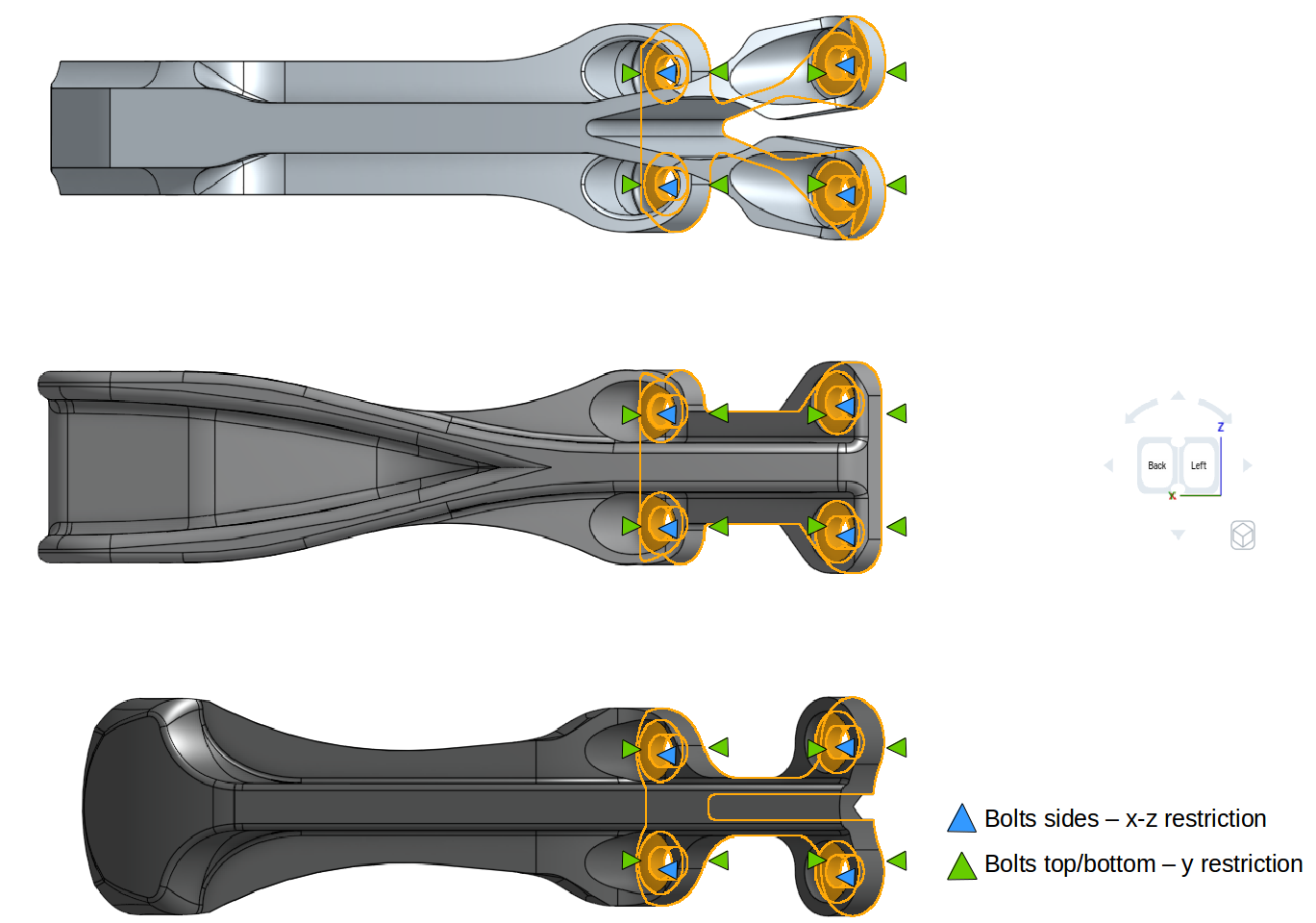
This exercise focus on the the testing of these three models based on the similar horizontal and vertical load provided in the GrabCAD challenge. In addition to this, the models were further tested considering the nonlinear plastic material and also increasing both loads. The applied constraint and loading boundary conditions are shown below. Please note that separate simulations were created for both loading types.

The different combinations for performing the simulations are:
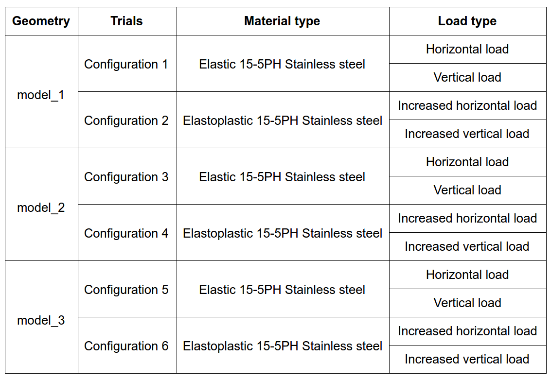
Please note that separate simulation needs to be set up for each configuration
Step-by-Step
Import the project by clicking the link below. (Crtl + Click to open in a new tab)
Click to Import the Homework Project
Meshing
-
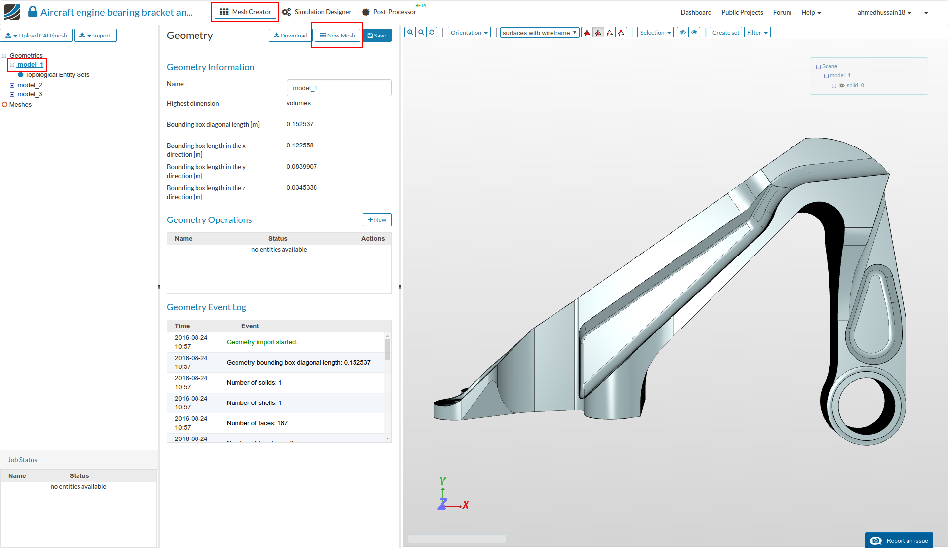
In the Mesh Creator tab, click on the geometry ‘model_1’
-
Then, click on ‘New Mesh’ button in the options panel.
- Change mesh order to Second order and ‘Number of computing cores’ to 8 cores. Click on ‘Start’ to start the meshing job. This operation will automatically create a mesh for the geometry. The meshing job will take some minutes to finish and show the status as Finished once done.
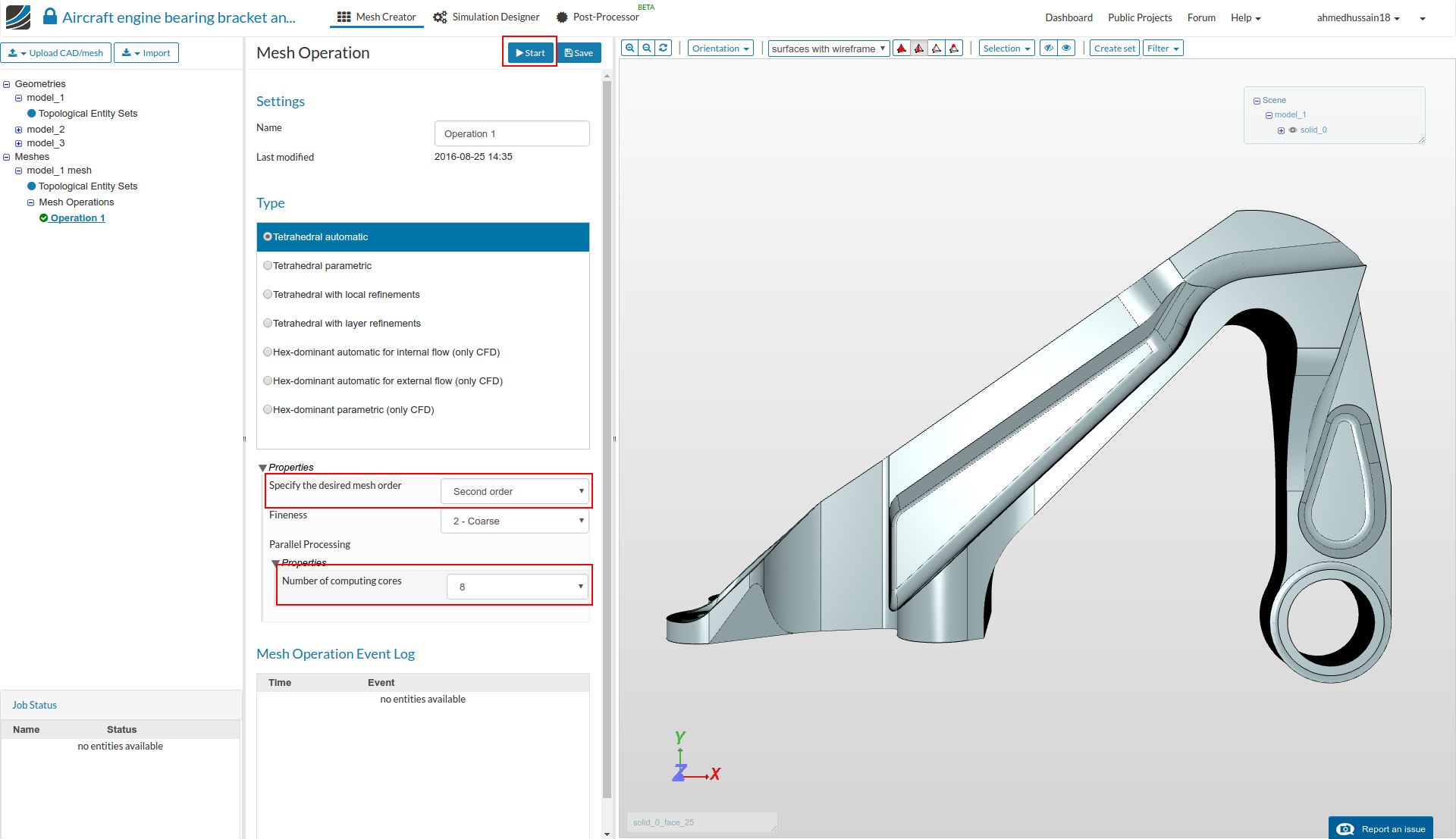
- Once finished, you will see the completed mesh in the viewer.

Follow the same procedure for all the other models
Simulation Setup
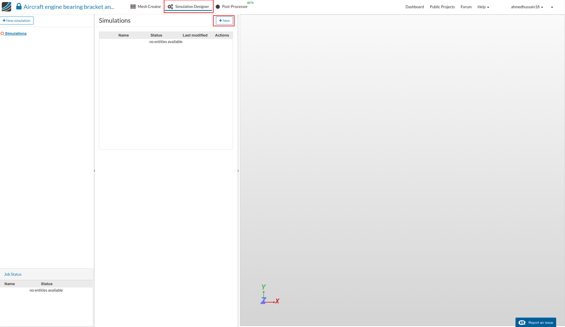
- For setting up the simulation switch to the Simulation Designer tab and click ‘New’ to create new simulation.
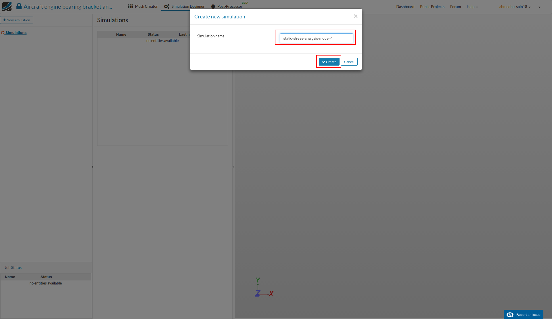
- A create new project window will pop-up. Give a project suitable name (optional) e.g. static-stress-analysis-model-1 in this case and click ‘Create’.
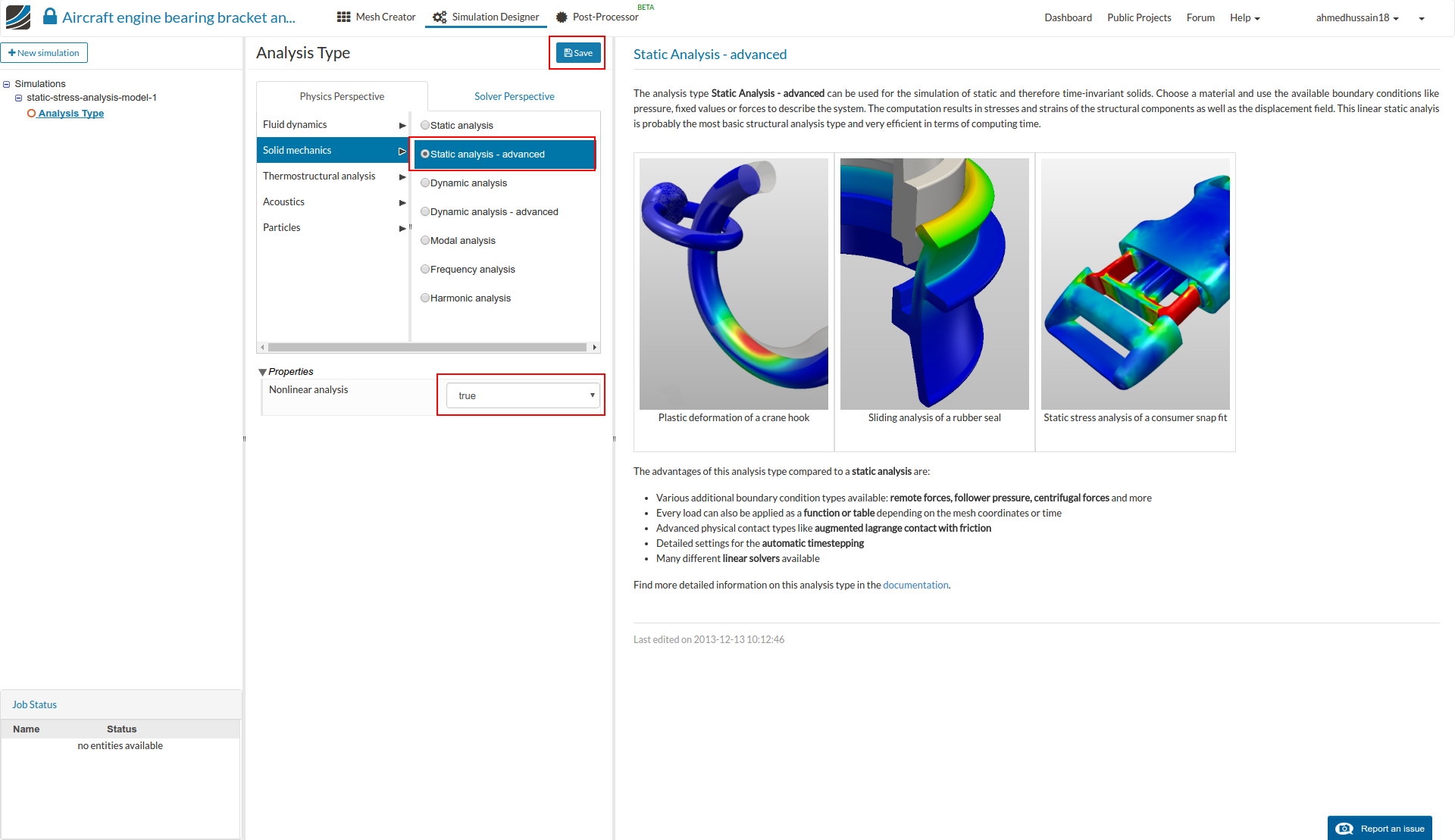
- Since our load will be static and later on we will be using a nonlinear material, we will select the analysis type ‘Static analysis - advanced’ under ‘Solid mechanics’, change the ‘Nonlinear analysis’ to true and click ‘Save’.
-
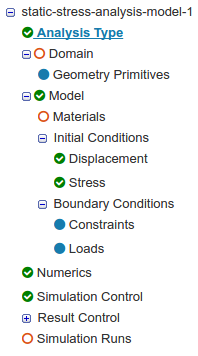
After saving, the simulation tree now looks as shown below. Here the ‘Tree Entries in Red’ must be completed.
Domain selection
- Click ‘Domain’ from the tree and select the first mesh created from the previous task. Click the ‘Save’ button. The mesh will then automatically load in the viewer.
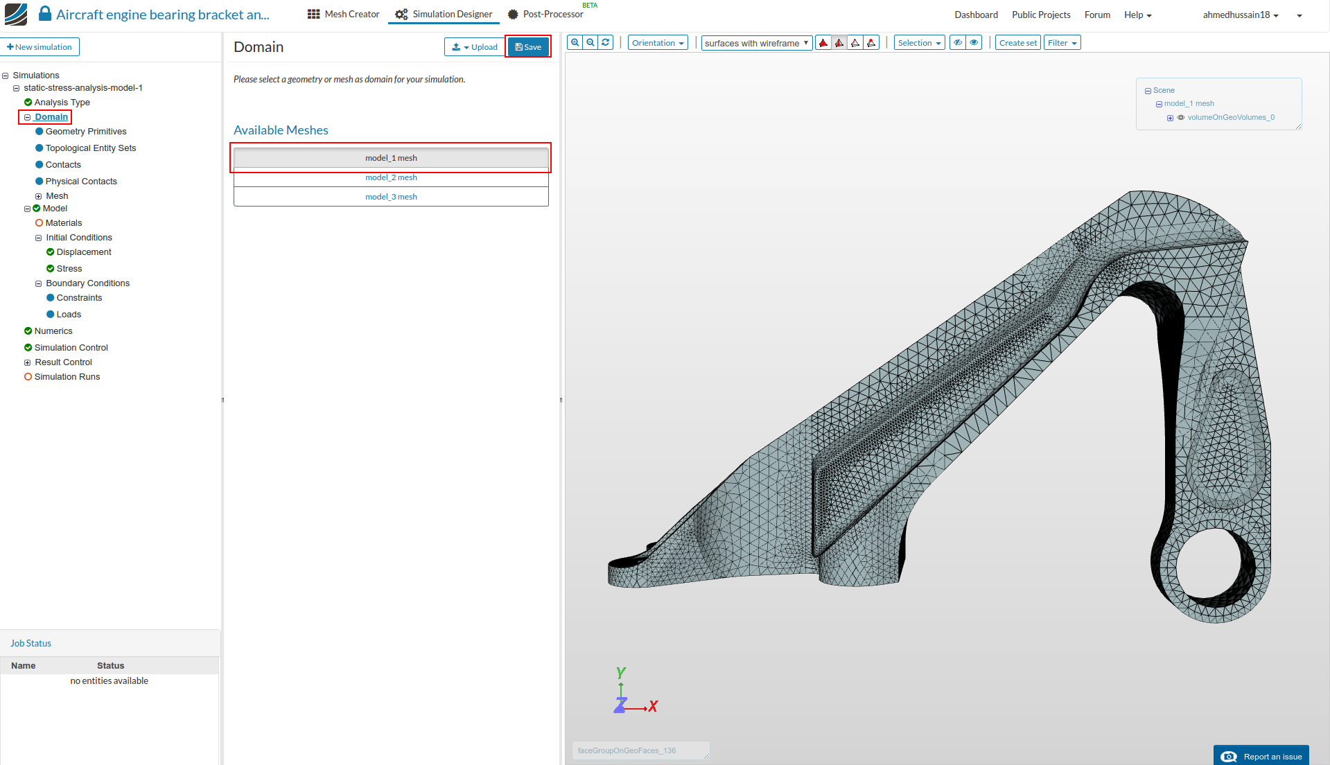
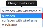
- Furthermore, change render mode to ‘Surfaces’ on viewer top to interact with the mesh more easily.
Topological Entity Sets
- For the ease we will create topological sets in order to use them further in our boundary conditions. The topological sets which we will create will be based on the figure below which explains all the boundary and loading conditions.
Constraints:

Loads:
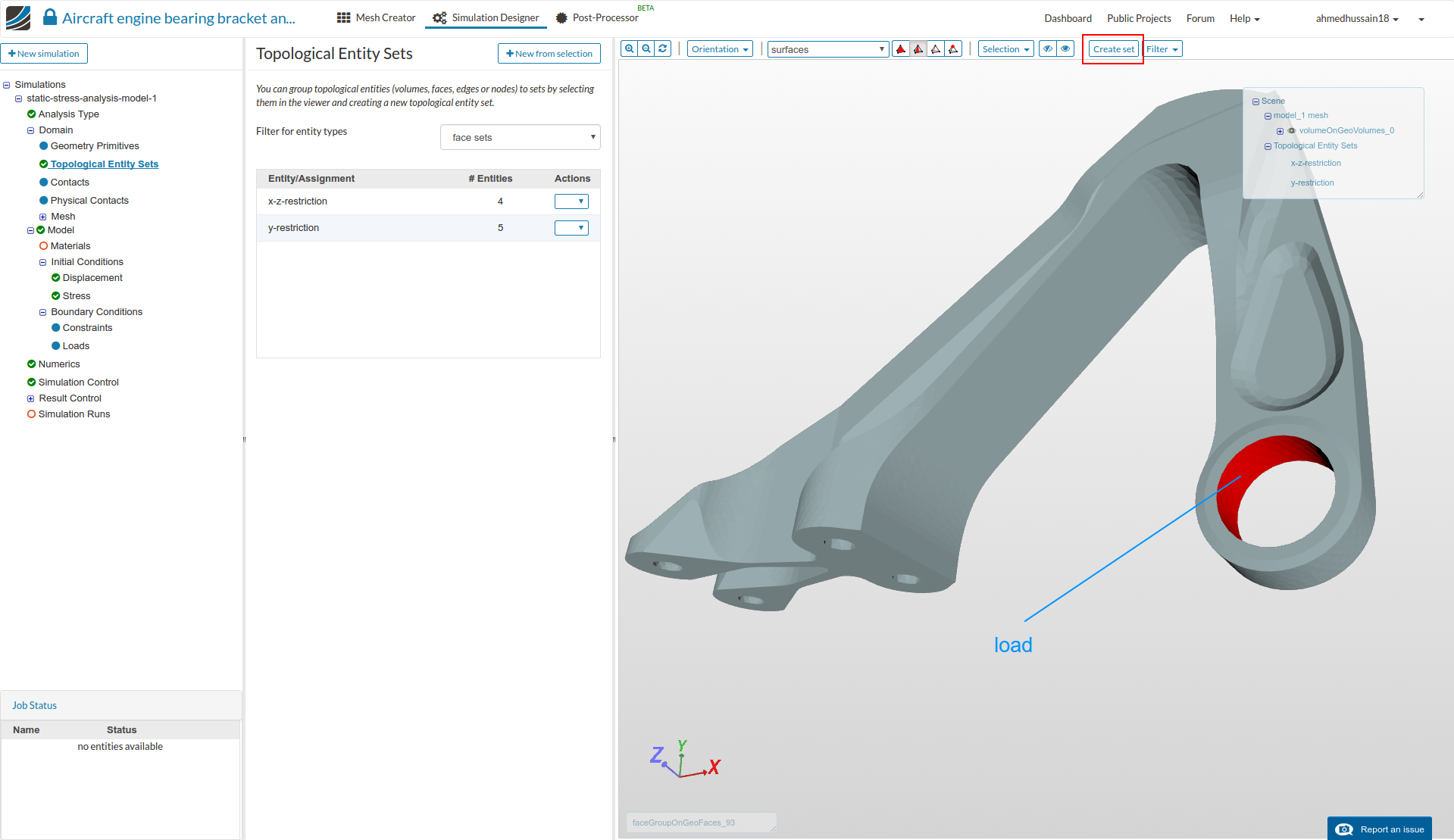
- We will create total of 3 topological entity sets as shown below:
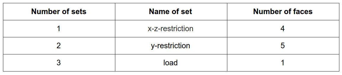
x-z-restriction
- Go to ‘Topological Entity Sets’, select the internal bolt faces of the geometry as shown in the figure below and then click ‘Create set’ on viewer top. Give set a reasonable name e.g. x-z-restriction in this case and click ‘Create set’ to create the set.
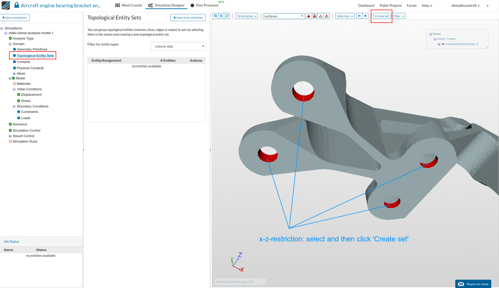
y-restriction
- Follow the same steps as above but this time select the upper and lower face of the geometry on bolt fixation as shown in the figure below. Give set a reasonable name e.g. y-restriction in this case and click ‘Create set’ to create the set.
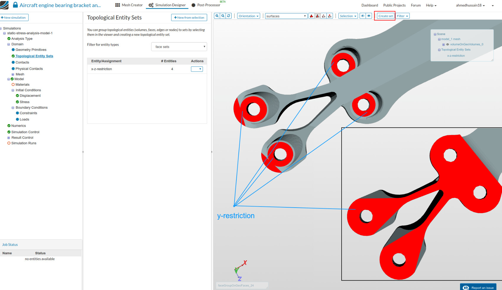
load
- Similarly, for the last topological set follow the same steps as above and this time select the internal face of the bearing front portion where the load will be applied. Give set a reasonable name e.g. load in this case and click ‘Create set’ to create the set.
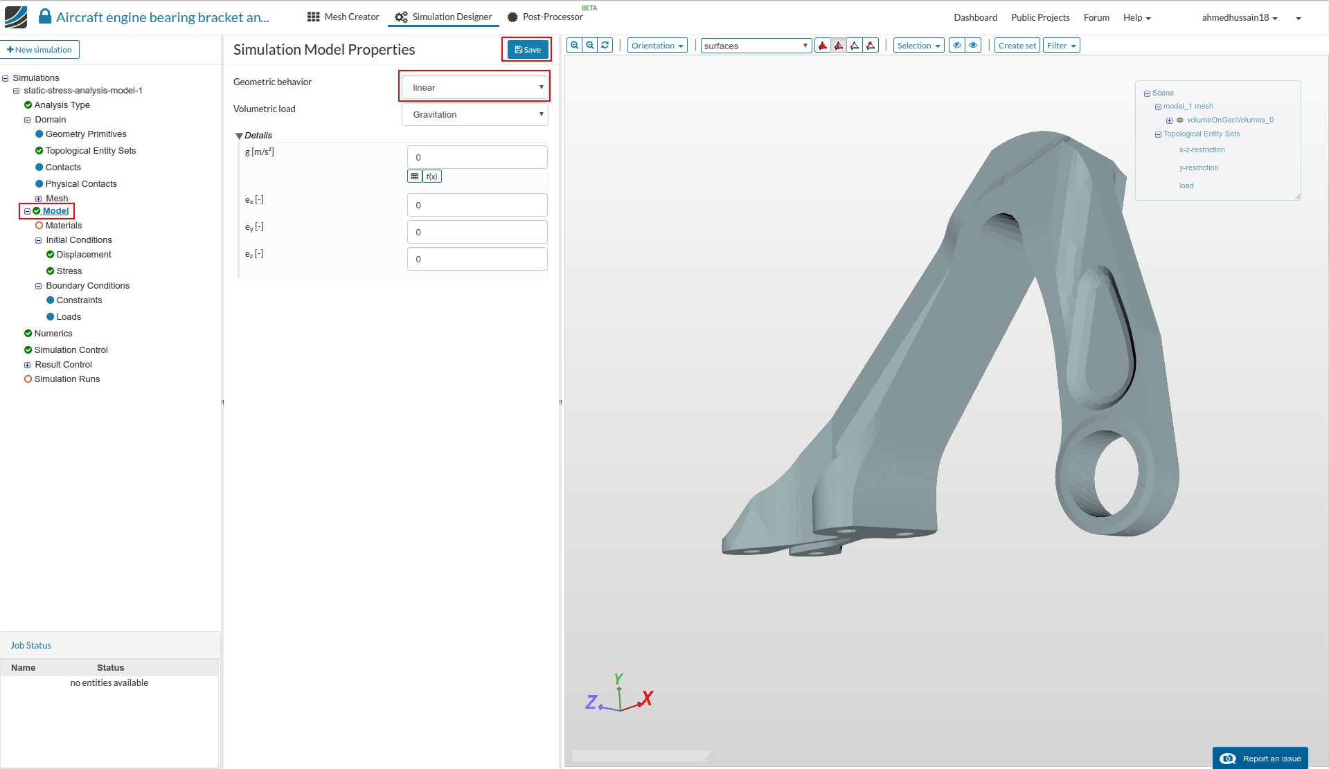
Model
- Due to small load conditions, turn off the geometric nonlinearity by going to ‘Model’ and setting ‘Geometric behavior’ to linear.
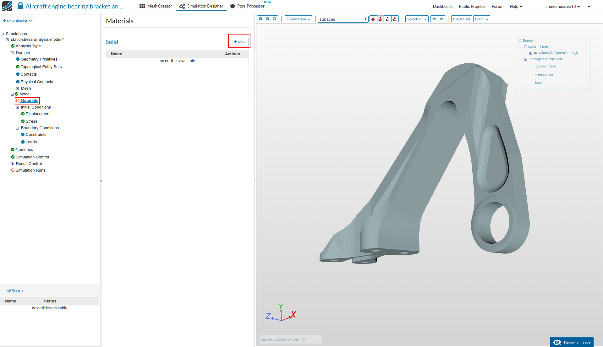
Materials
-
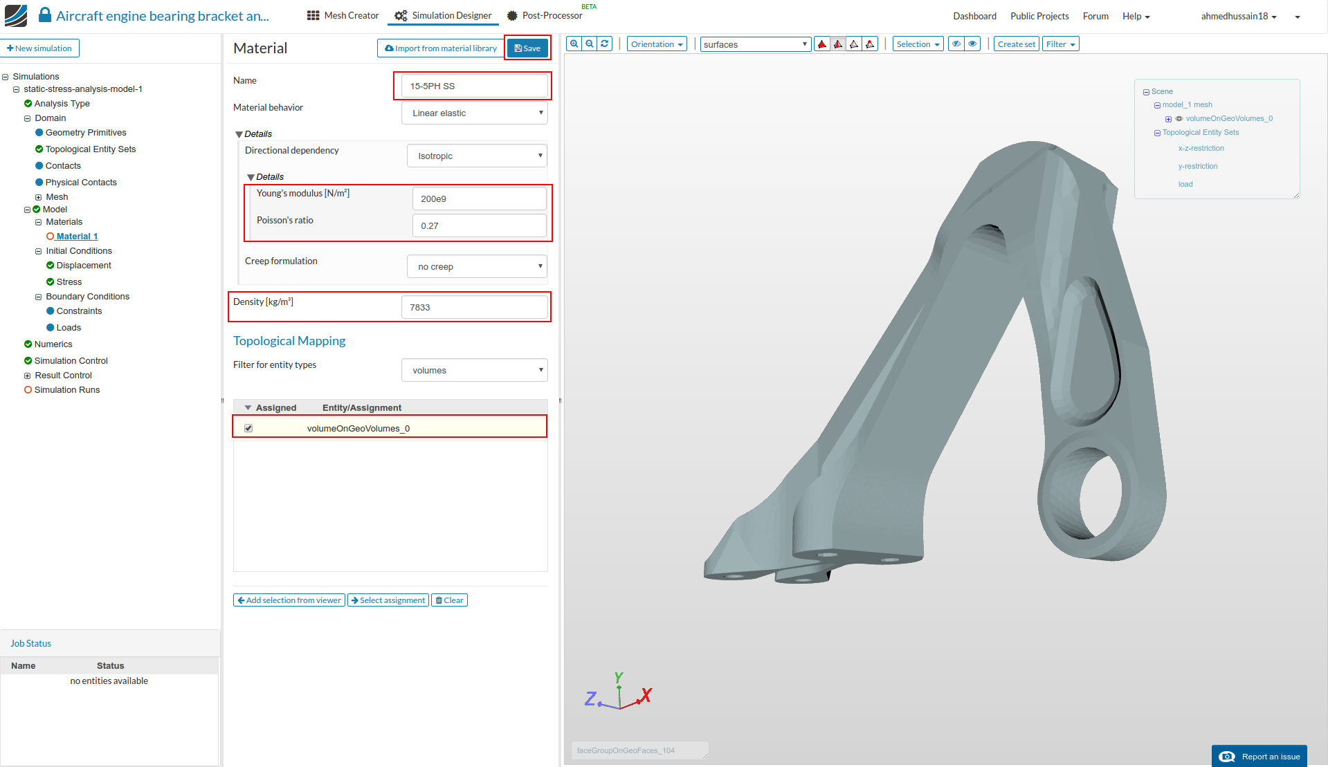
For the ‘Configuration 1’ we have to only define an elastic material for our bearing bracket. The material we will be going to use is ‘15-5PH Stainless steel’ which is a fairly tough material with high yield strength of ‘1 GPa’.
-
In order to define a material, go to ‘Materials’ under tree and click ‘New’ to create new material definition.
- Rename newly created material to 15-5PH SS (optional). Change the ‘Young’s modulus’, ‘Poisson’s ratio’ and ‘Density’ values to 200e9, 0.27 and 7833 as shown in figure below. Select the volumeOnGeoVolumes_0 under ‘Topological Mapping’ and click ‘Save’ in order to assign the material to the geometry.
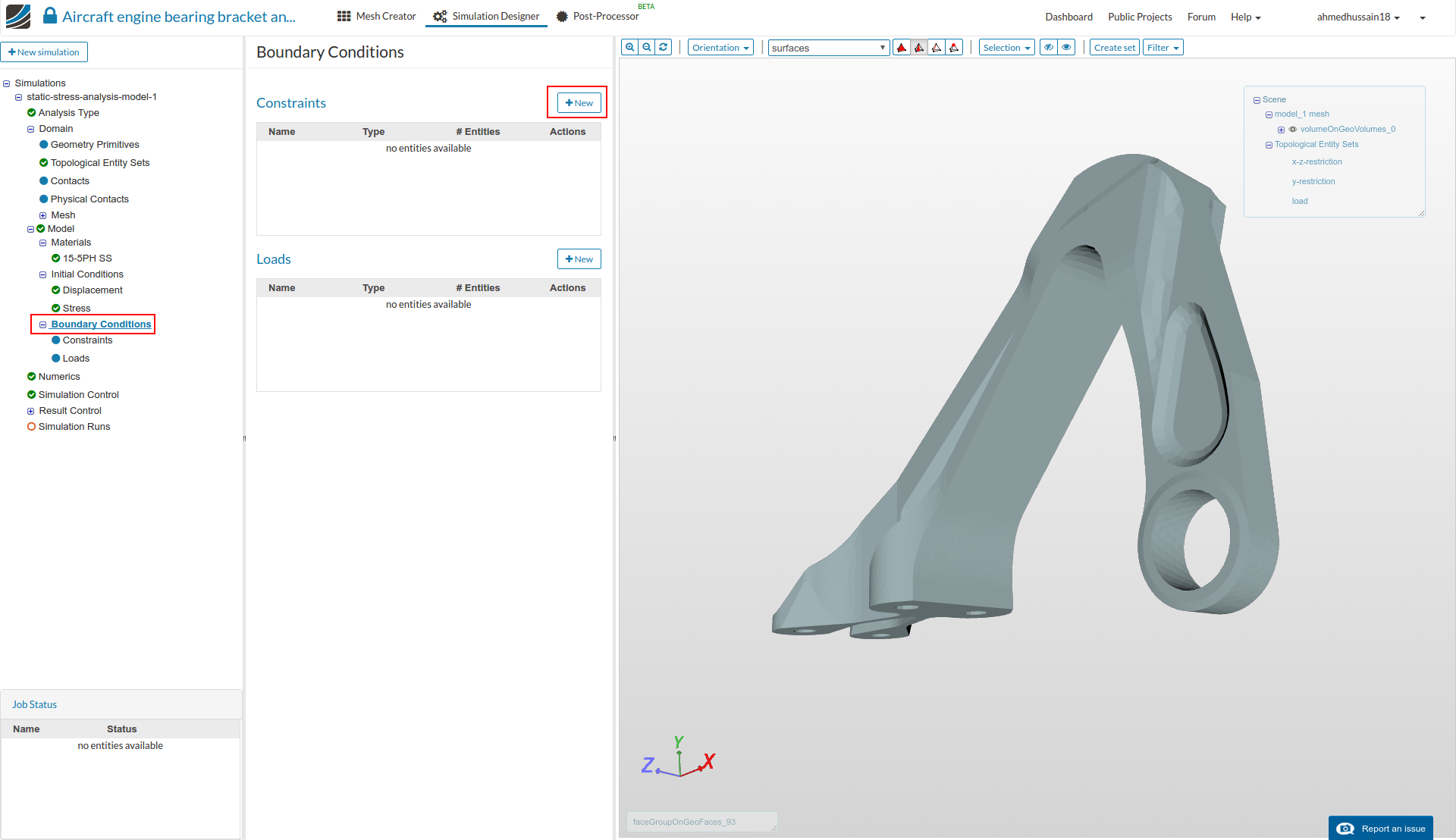
Boundary Conditions
-
Now we will proceed with the constraint and load definitions for our simulation case, as discussed before.
-
Go to ‘Boundary Conditions’ under simulation tree and click ‘New’ next to constraint to define the symmetry boundary conditions.
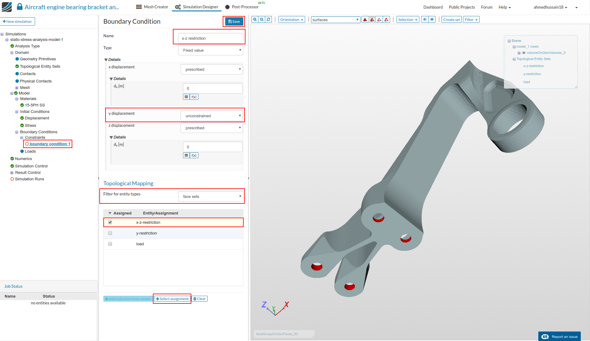
x-z restriction:
-
We now have to define restriction along x-z axis so that the geometry shouldn’t be allowed to move along x-z axis mimicking the same behavior as bolts are restricting this motion. Rename the newly created boundary condition to x-z restriction (optional). Set only ‘y displacement’ to unconstrained.
-
Change ‘Filter for entity types’ to face sets under ‘Topological Mapping’ and select ‘x-z-restriction’, click ‘Select assignment’ to see highlight the selected assignment in viewer. Click ‘Save’ to save the constraint.
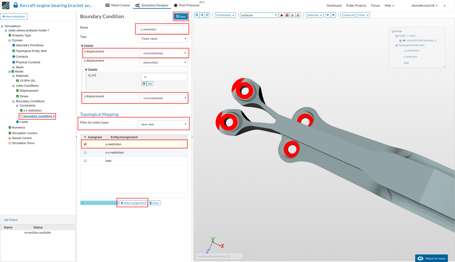
y restriction:
-
We now have to define restriction along y axis so that the geometry shouldn’t be allowed to move along y axis mimicking the same behavior as bolts are restricting the pulling out of geometry from the base it is connected to. Do the same process as before and rename the newly created boundary condition to y restriction (optional). This time set both ‘x displacement’ and ‘z displacement’ to unconstrained.
-
Change ‘Filter for entity types’ to face sets under ‘Topological Mapping’ and select ‘y-restriction’, click ‘Select assignment’ to see highlight the selected assignment in viewer. Click ‘Save’ to save the constraint.
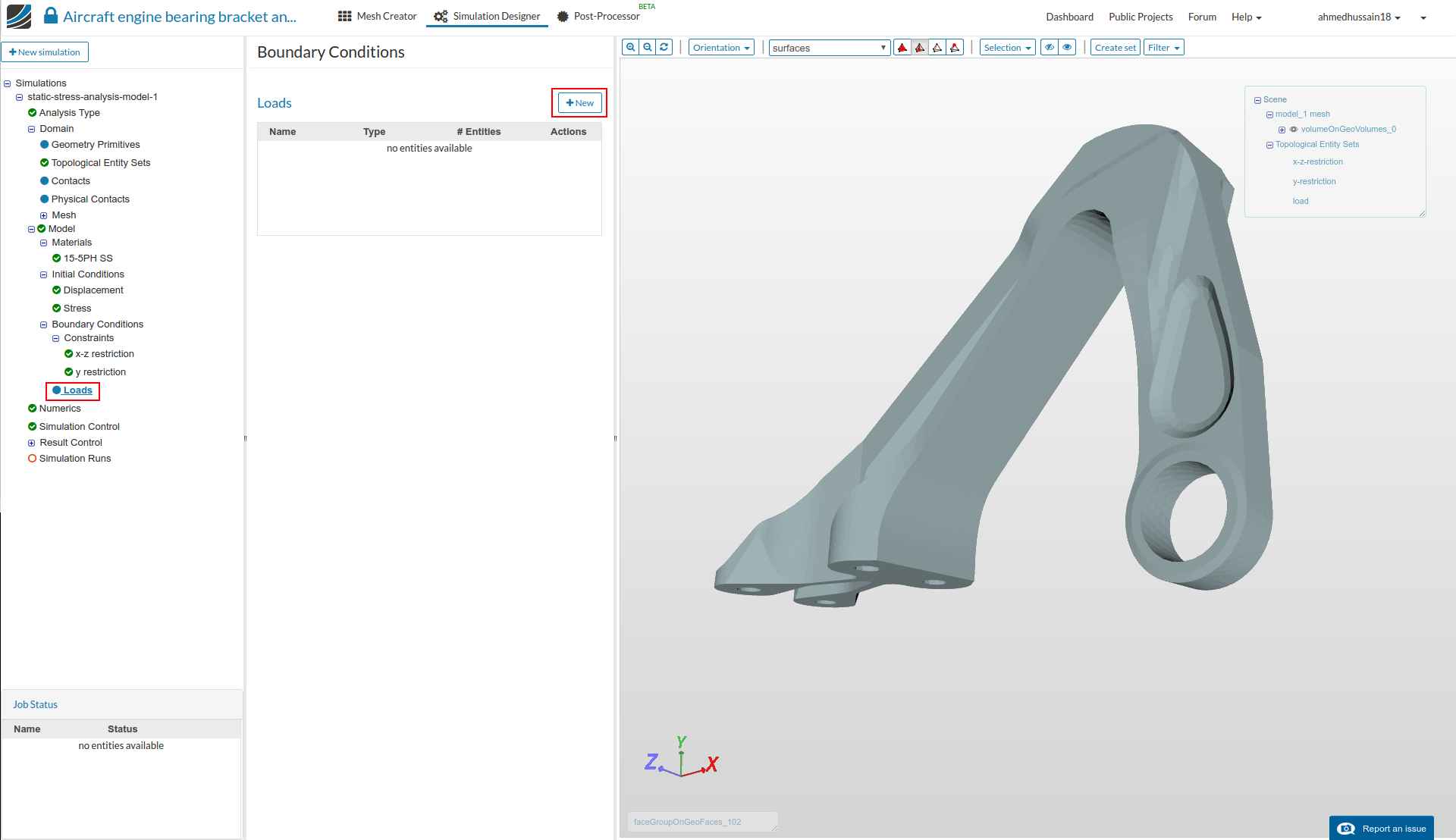
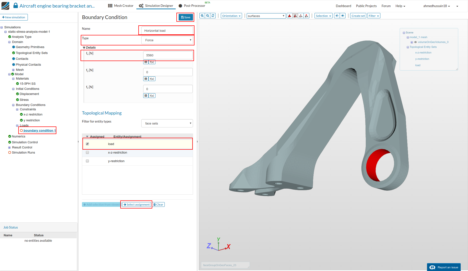
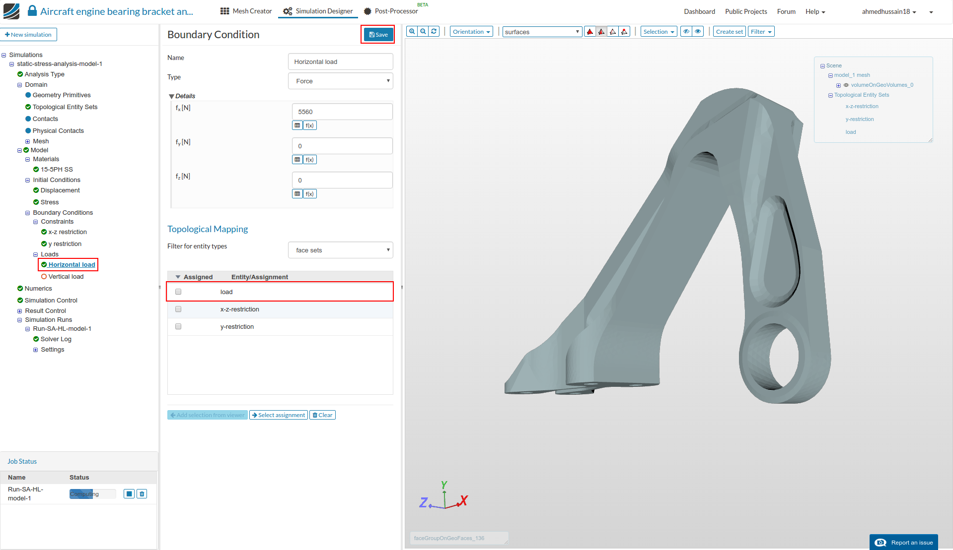
Horizontal load:
- Next we will define our horizontal load boundary condition. Proceed to ‘Loads’ under tree and click ‘New’ to create a new load definition.
-
Rename the newly created constraint to Horizontal load (optional). Change ‘Type’ to Force and give value of 5560 next to ‘fx[N]’.
-
Next select ‘load’ under ‘Topological Mapping’, click ‘Select assignment’ to see highlight the selected assignment in viewer. Click ‘Save’ to save the load definition. (Ignore the warning that pops-up)
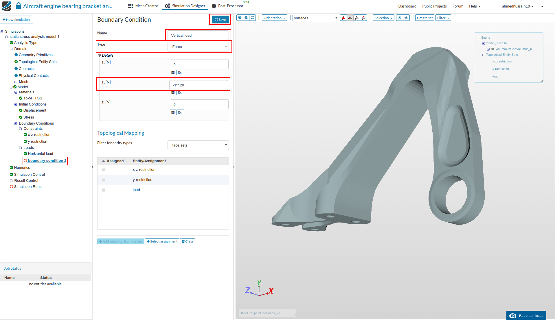
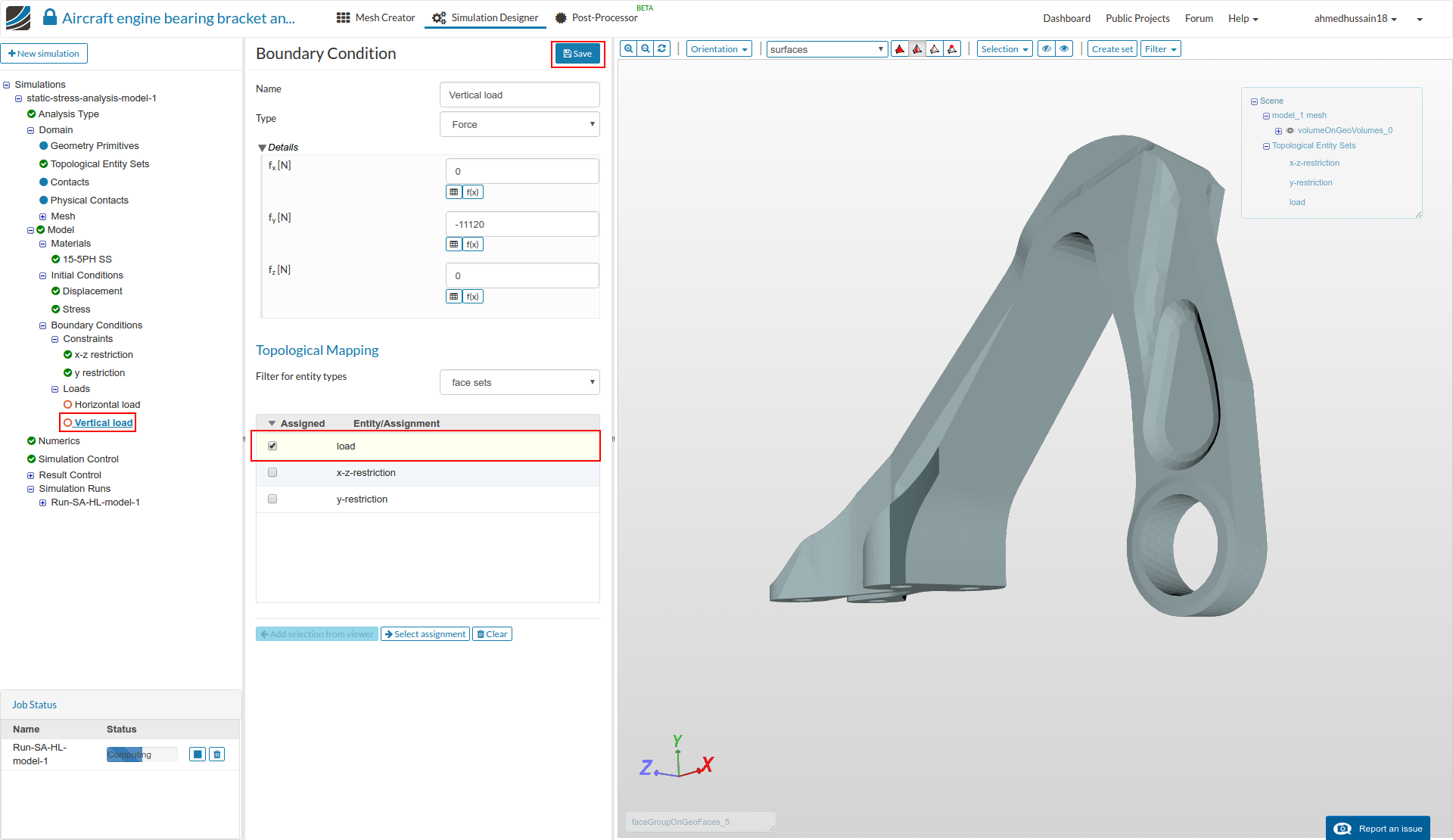
Vertical load:
-
Follow the same procedure as above. Rename the newly created constraint to Vertical load (optional). Change ‘Type’ to Force and give value of -11120 next to ‘fy[N]’. Click ‘Save’ to save the load definition.
-
Don’t select any ‘Topological Mapping’ this time as we have created this for our next simulation run. Click ‘Save’ to save the load definition.
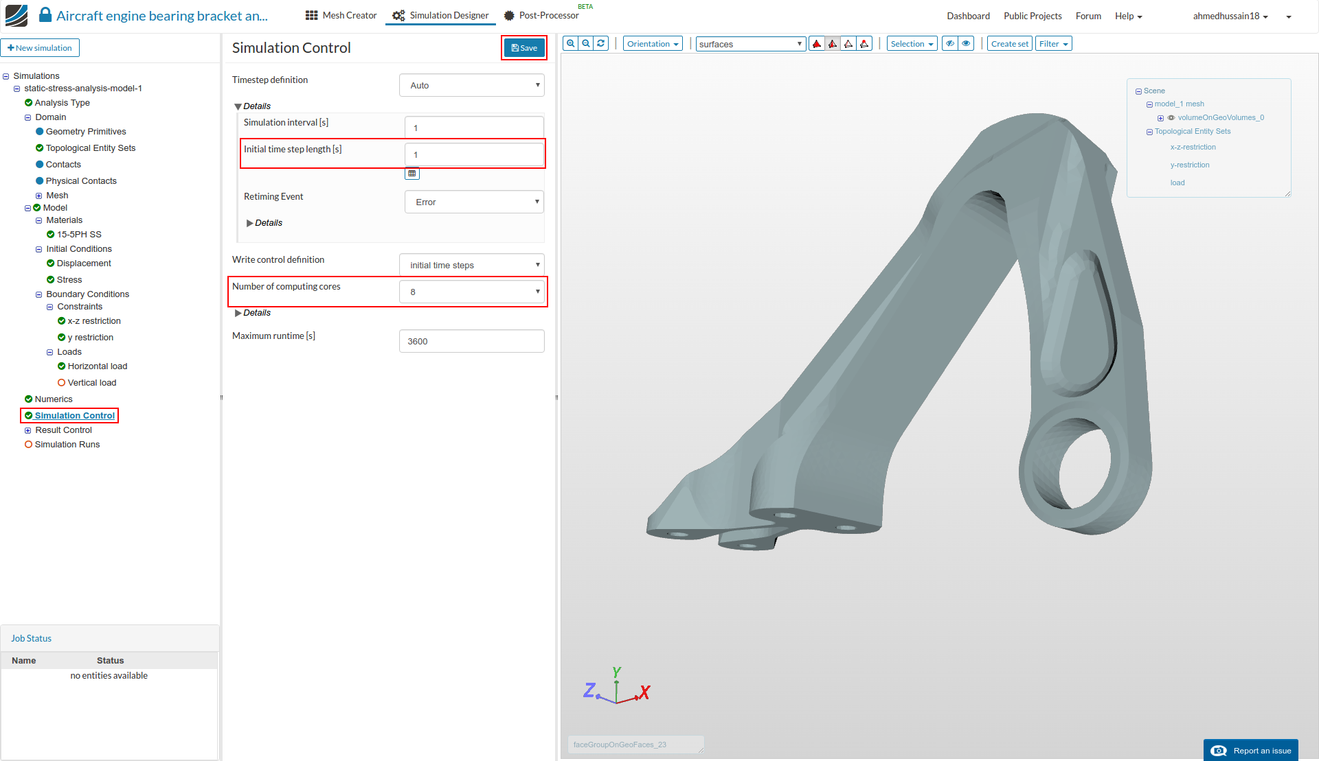
Simulation Control
- Click on Simulation control and change ‘Initial time step length [s]’ to 1 (as this is a linear static analysis therefore one analysis step would be enough) , ‘Number of computing cores’ to 8. Click ‘Save’ to register the changes.
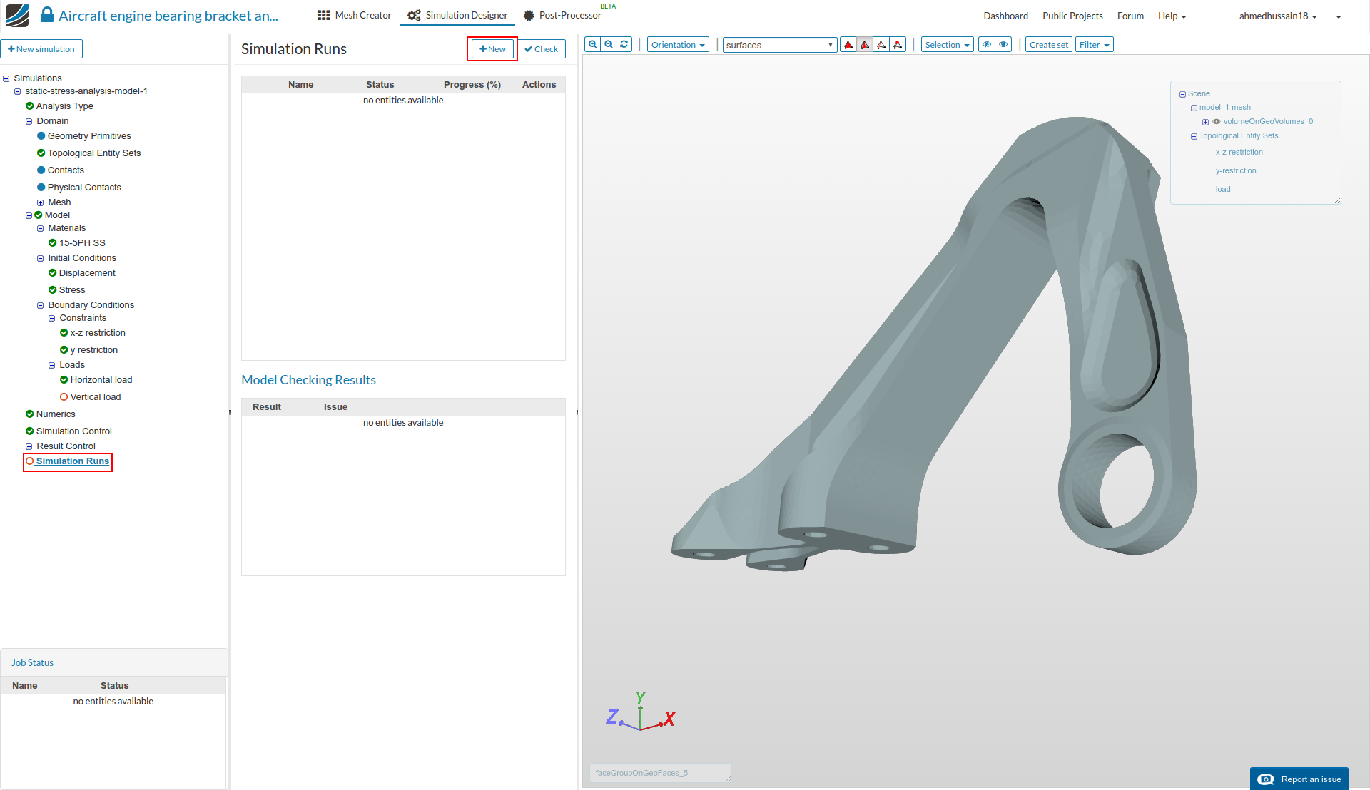
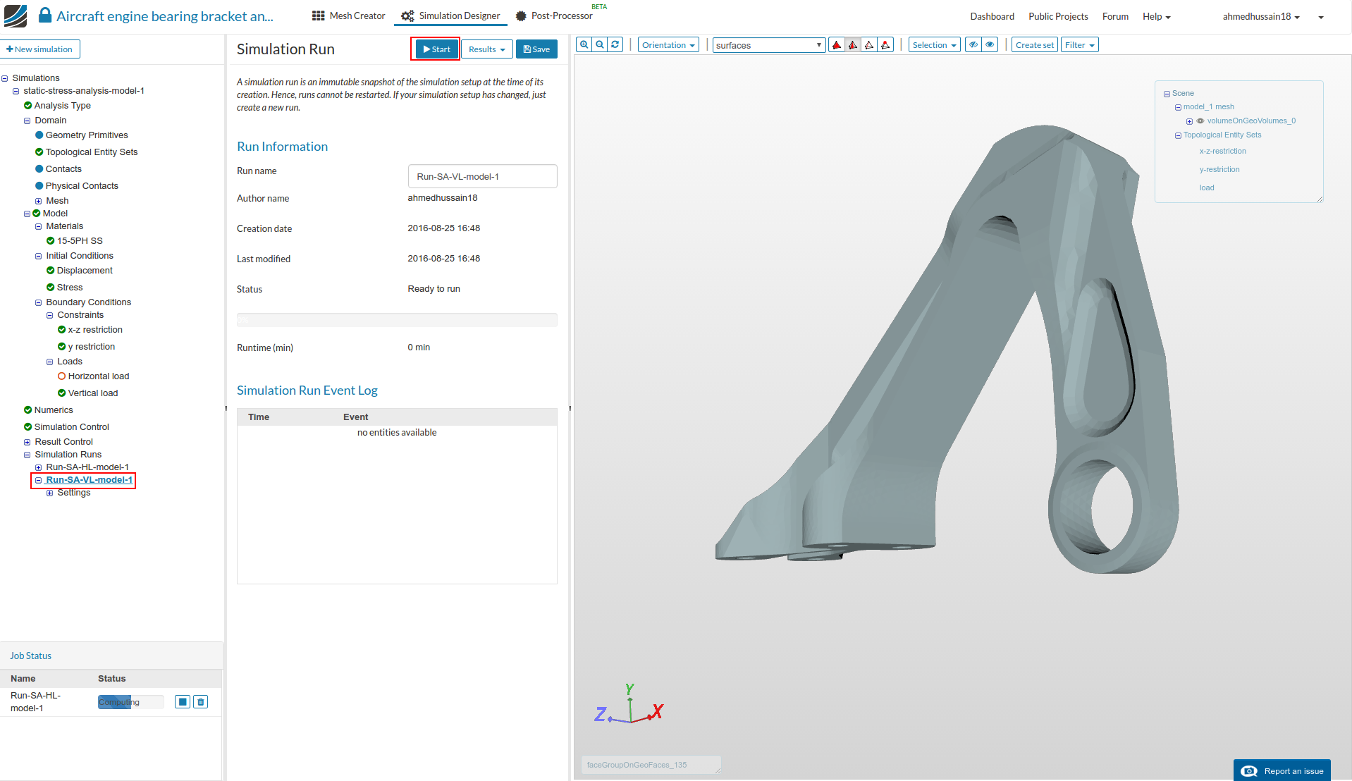
Simulation Run
- All good for creating our first simulation run. Go to Simulation runs and create a ‘New’ run. Give simulation run a suitable name in the pop-up window that appears e.g. Run-SA-HL-model-1 (optional) in this case. Click ‘Create’ to create a new run. (Ignore the warnings that pops-up)
- The new run will be created under ‘Simulation Runs’. Click ‘Start’ to run the simulation.
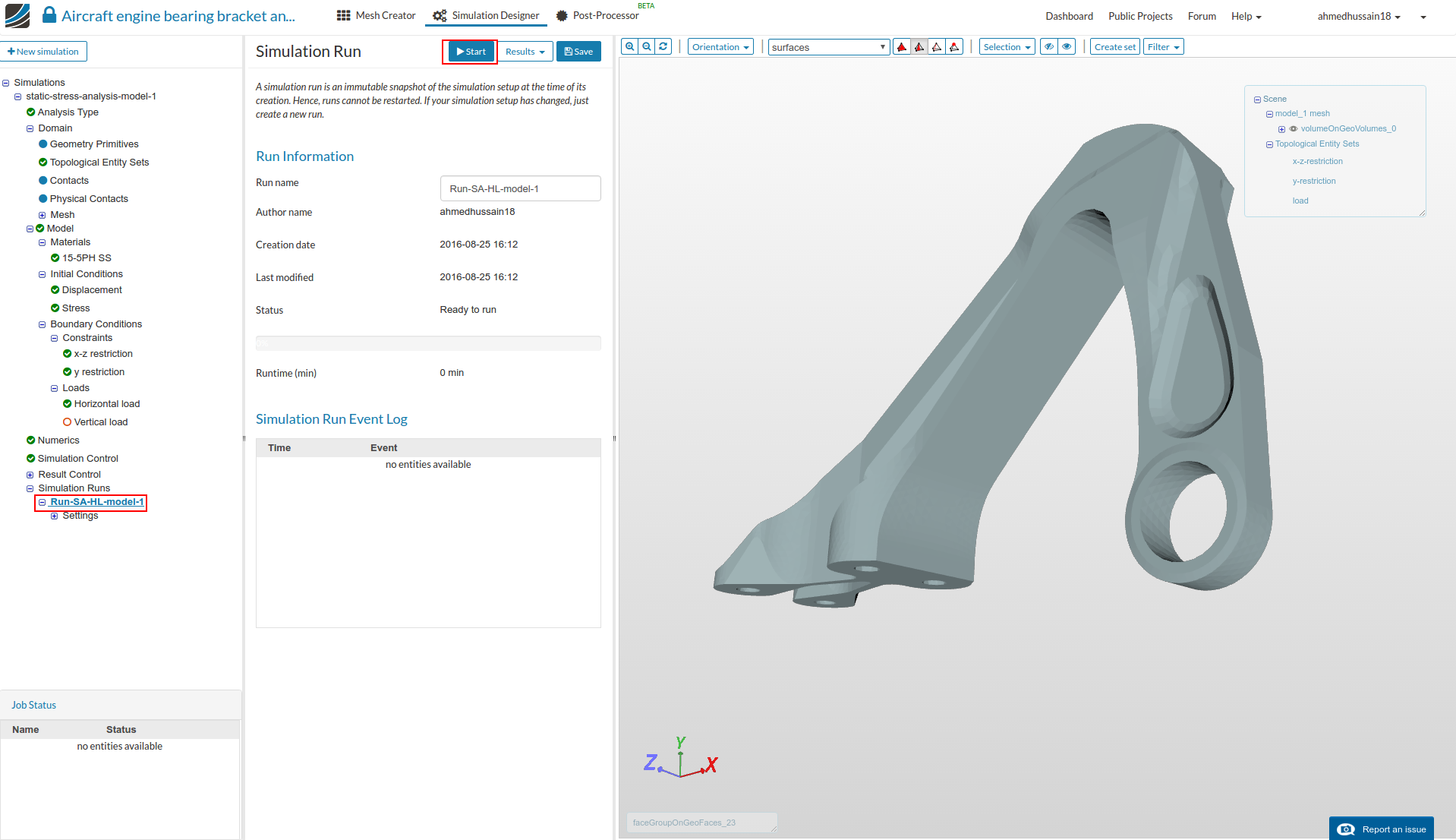
- The simulation run will take approx. 8 min. to finish.
Vertical load case
- For applying the vertical load, go to ‘Horizontal load’ un-check ‘load’ under ‘Topological Mapping’ and click ‘Save’.
- Next go to ‘Vertical load’ and check ‘load’ under ‘Topological Mapping’ and click ‘Save’. (Ignore the warning that pops-up)
- Go to Simulation runs and create a ‘New’ run. Give simulation run a suitable name in the pop-up window that appears e.g. Run-SA-VL-model-1 (optional) in this case. Click ‘Create’ to create a new run. (Ignore the warnings that pops-up)
Create Further Configurations
Configuration 2:
-
Once you have started all the runs with the first configuration setup, go ahead and make a duplicate of this simulation in order to perform the simulation with different material type for hip joint (configuration 2).
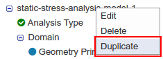
-
Rename the simulation to static-nonlinear-stress-analysis-model-1 and click ‘Save’.
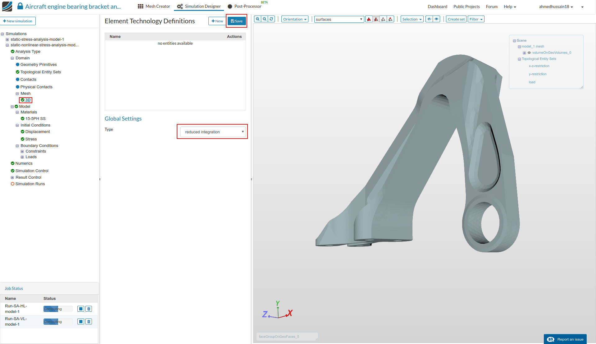
Mesh element technology definition
- Since we are going to deal with a plastic material using second order elements, it’s always recommended to use ‘reduced integration’ element technology to get the more realistic results. In order to do so, go to ‘3D’ tree under ‘Mesh’ option and change ‘Type’ from standard to reduced integration. Click ‘Save’ to register changes.
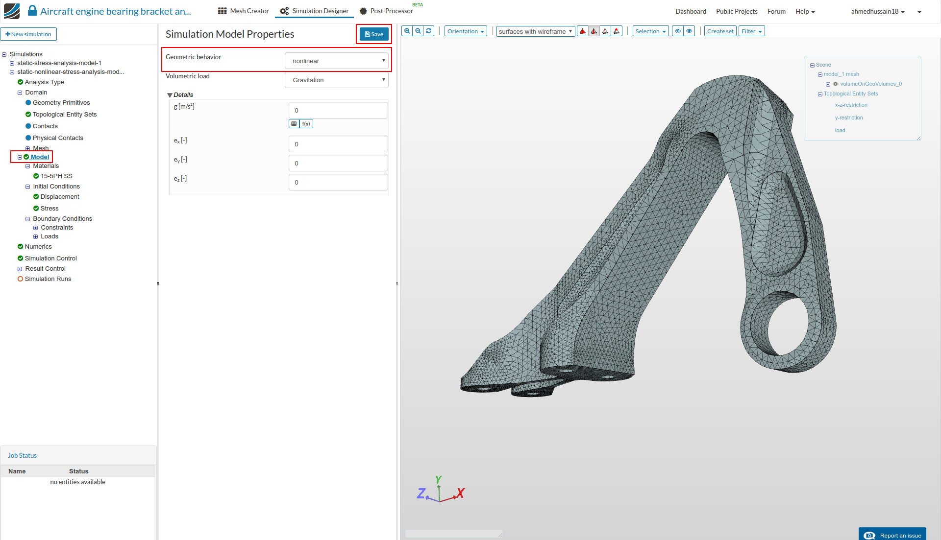
Model
- Due to large load conditions, we will now turn back to the geometric nonlinearity by going to ‘Model’ and setting ‘Geometric behavior’ to nonlinear.
Materials
-
Now we will define a plastic material for which we have to first create a .csv file with our plastic material data. The stress strain data in this .csv file will start from yield point of 15-5PH stainless steel. Just copy the values given below, create a new ‘Notepad’ (or any notepad application) file on your computer and paste them there. Save the file by first changing the file types to all rather than ‘.txt file’ or some other. Then give it some reasonable name e.g. 15-5PH-SS-stress-strain.csv in this case and click ‘Save’. (material data is taken from [1])
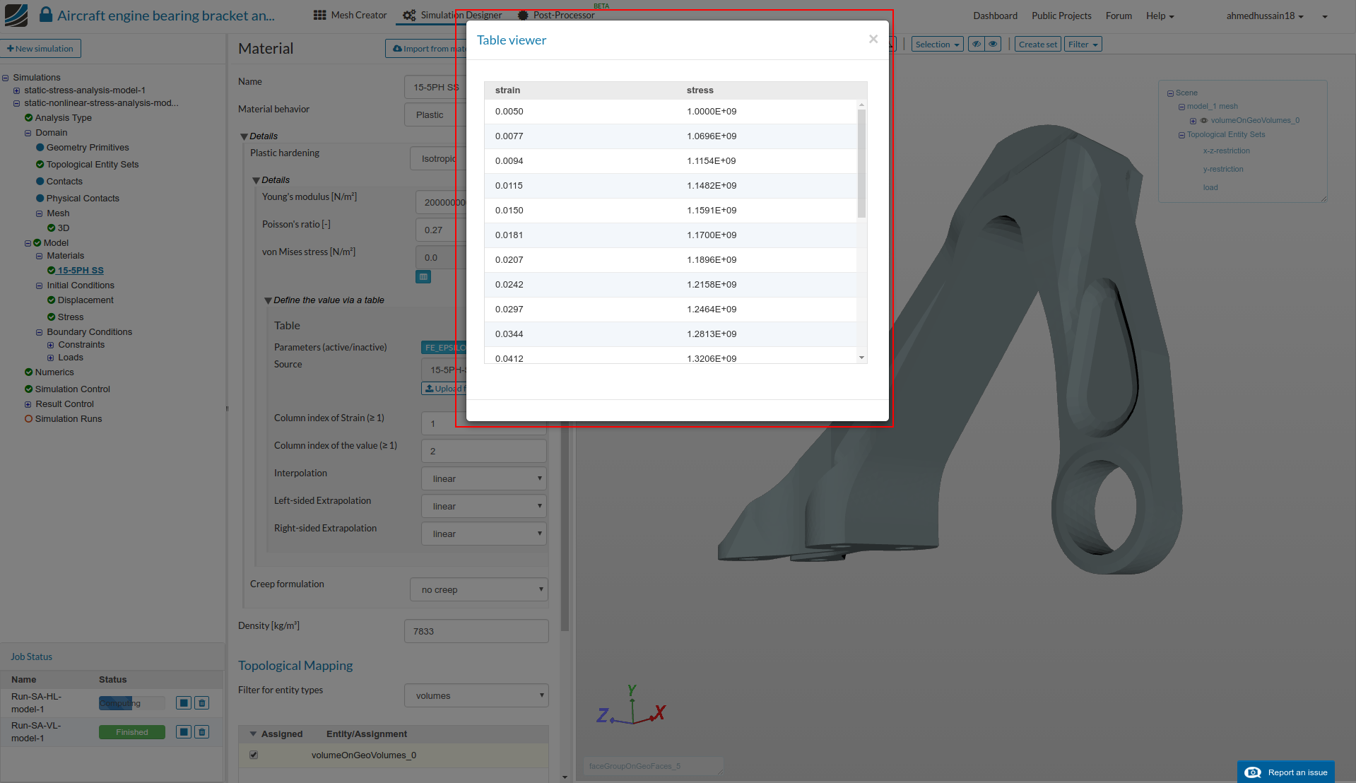
strain,stress
0.0050 ,1.0000E+09
0.0077,1.0696E+09
0.0094,1.1154E+09
0.0115,1.1482E+09
0.0150,1.1591E+09
0.0181,1.1700E+09
0.0207,1.1896E+09
0.0242,1.2158E+09
0.0297,1.2464E+09
0.0344,1.2813E+09
0.0412,1.3206E+09
0.0488,1.3643E+09
0.0570,1.4057E+09
0.0663,1.4450E+09
0.0755,1.4690E+09
0.0849,1.4756E+09
0.0962,1.4603E+09
0.1049,1.4254E+09
0.1144,1.3774E+09
0.1226,1.3315E+09
0.1301,1.2791E+09
0.1367,1.2289E+09
0.1431,1.1787E+09
0.1495,1.1154E+09 -
After creating the file, go back to simulation and then go to ‘15-5PH SS’ under ‘Materials’ and change ‘Material behavior’ to Plastic. Change ‘Young’s modulus’ and ‘Poisson’s ratio’ to 200e9 and 0.27 respectively.
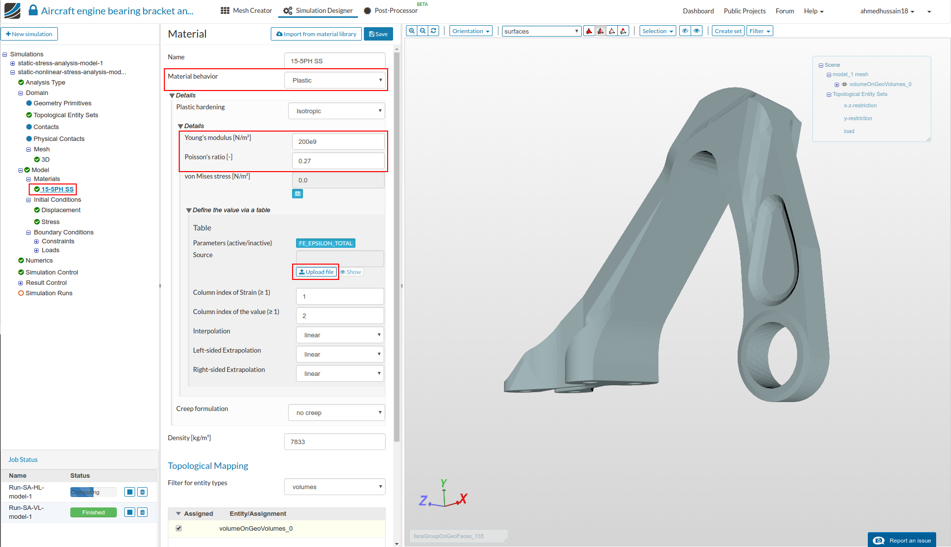
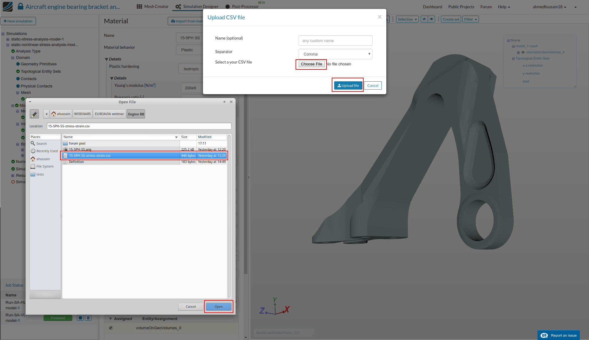
- Upload the created file by clicking ‘Upload file’ as shown in the figure of previous step to upload it. A pop-up window will open, click ‘Choose file’ and open your created file from your computer and then click ‘Upload file’ as shown in the figure below.
- Click ‘Save’ to save the new material definition.
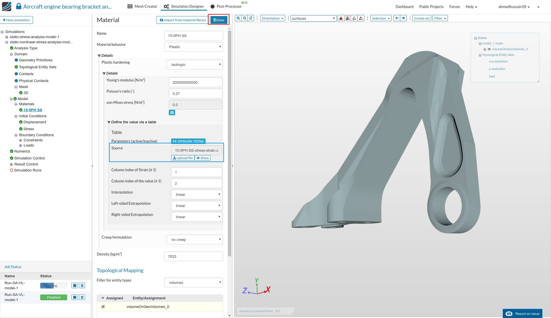
- You can click ‘Show’ to see the material data which should look something like this:
Loads
-
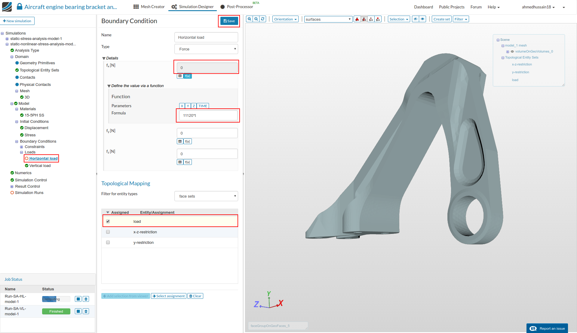
Next go to ‘Horizontal load’ and change value of ‘fx[N]’ back to zero and click small ‘f(x)’ below it. Give the value of 11120*t which will ramp the load over time (as solver doesn’t perform this automatically) and material nonlinearity will solved easily.
-
Select ‘load’ under ‘Topological Mapping’ and click ‘Save’ to register your changes.
-
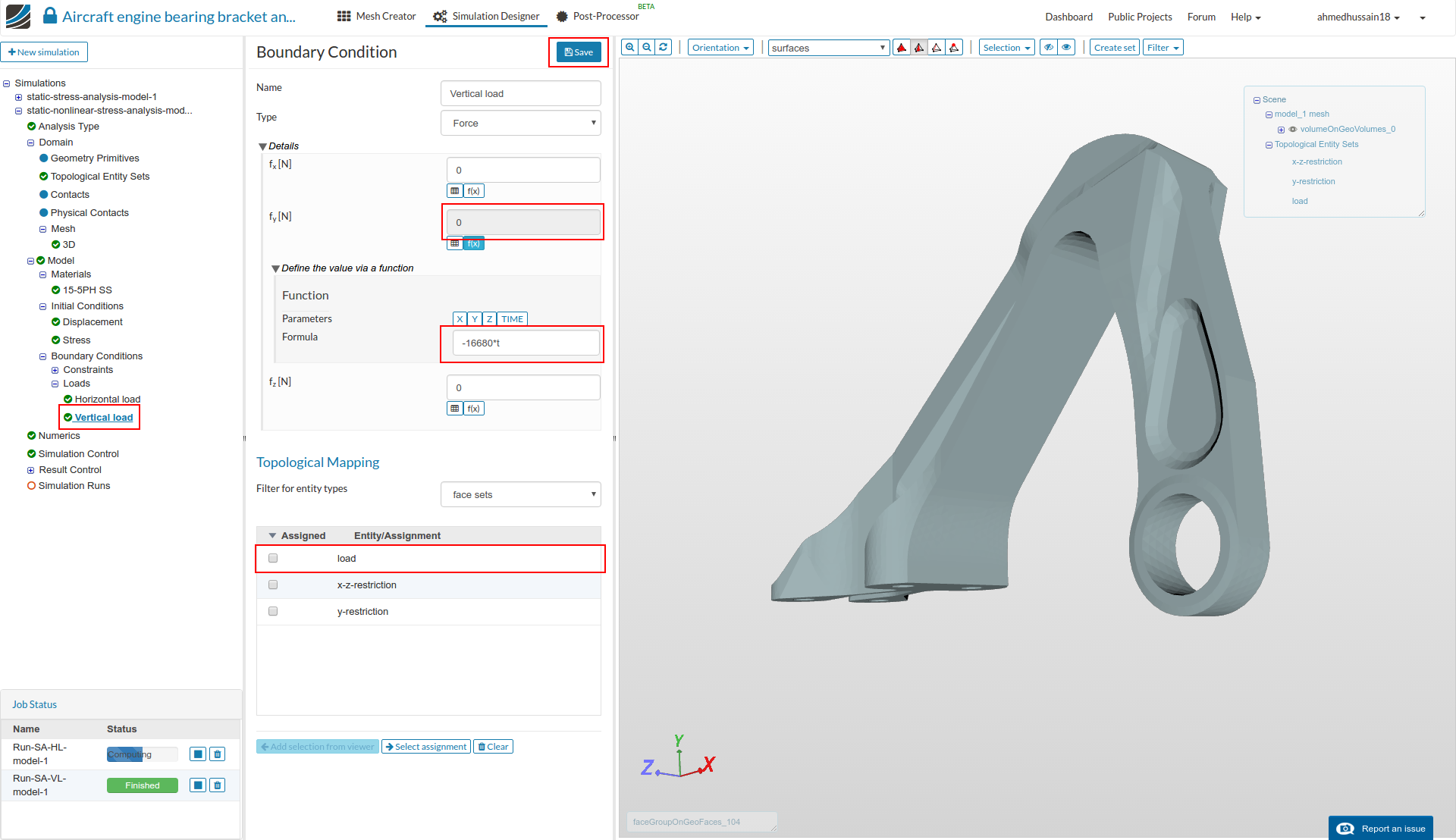
Next go to ‘Vertical load’ and change value of ‘fy[N]’ back to zero and click small ‘f(x)’ below it. Give the value of -16680*t.
-
Deselect ‘load’ under ‘Topological Mapping’ and click ‘Save’ to register your changes.
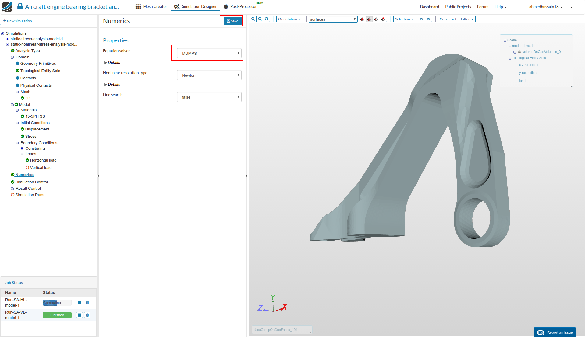
Numerics
- Go to ‘Numerics’ under the simulation tree, change ‘Equation Solver’ to MUMPS which is a faster solver for nonlinear problems. Click ‘Save’ to save the changes.
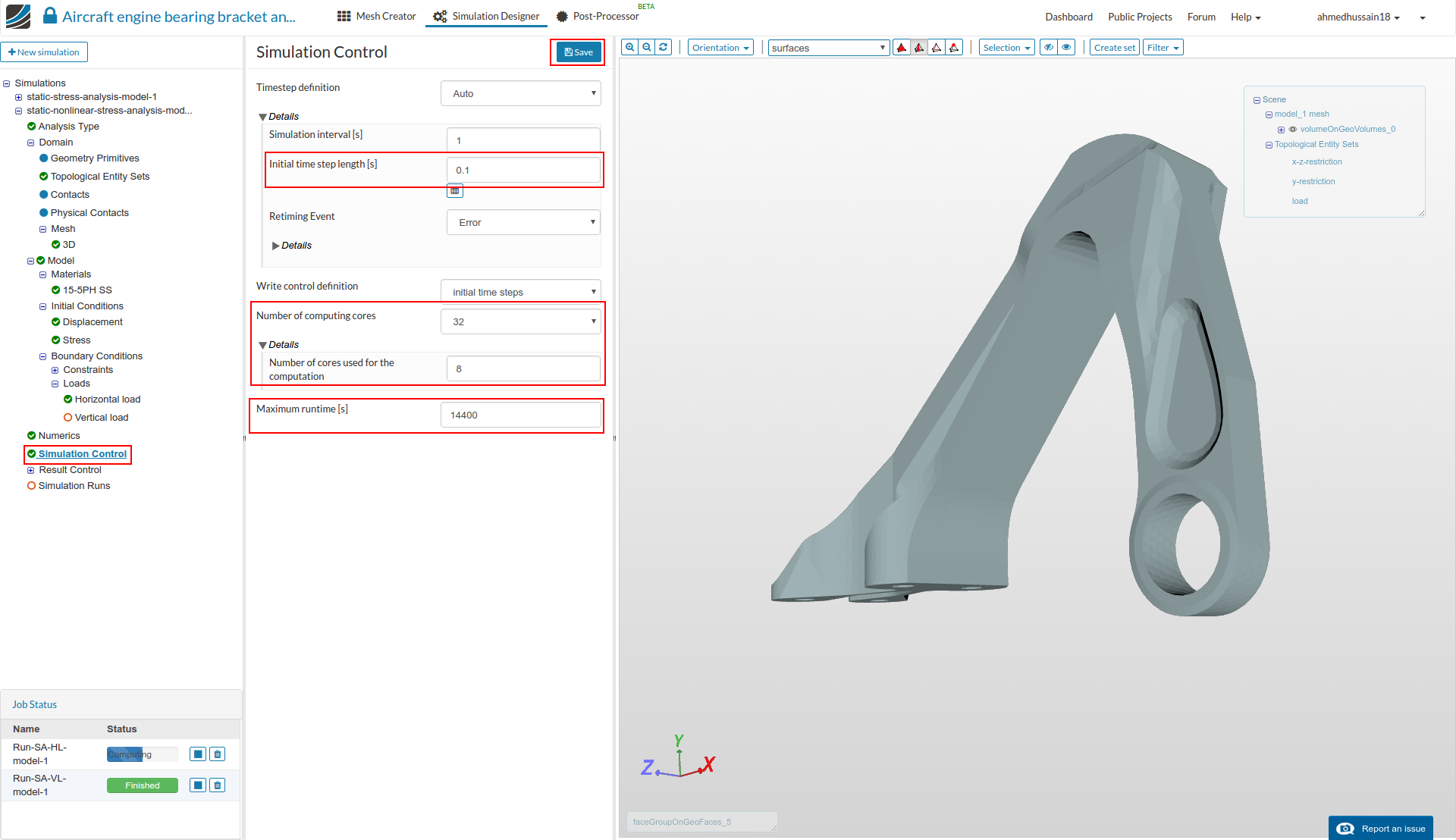
Simulation Control
- Go to ‘Simulation Control’ and change ‘Initial time step length [s]’ to 0.1, ‘Number of computing cores’ to 32, ‘Number of cores used for the computation’ to 8 and ‘Maximum runtime [s]’ to 14400. Click ‘Save’ to register changes.
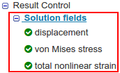
Result Control
-
Go to ‘Solution fields’ under ‘Result Control’ and delete ‘cauchy stress’ which will later on save computation time.
-
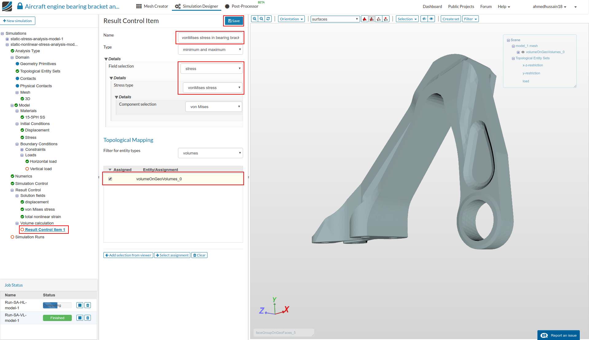
Next click ‘Result Control’ in simulation tree and click ‘New’ in front of ‘Volume calculation’ to create a new volume calculation method which will plot the minimum and maximum vonMises stress of a volume later in results.
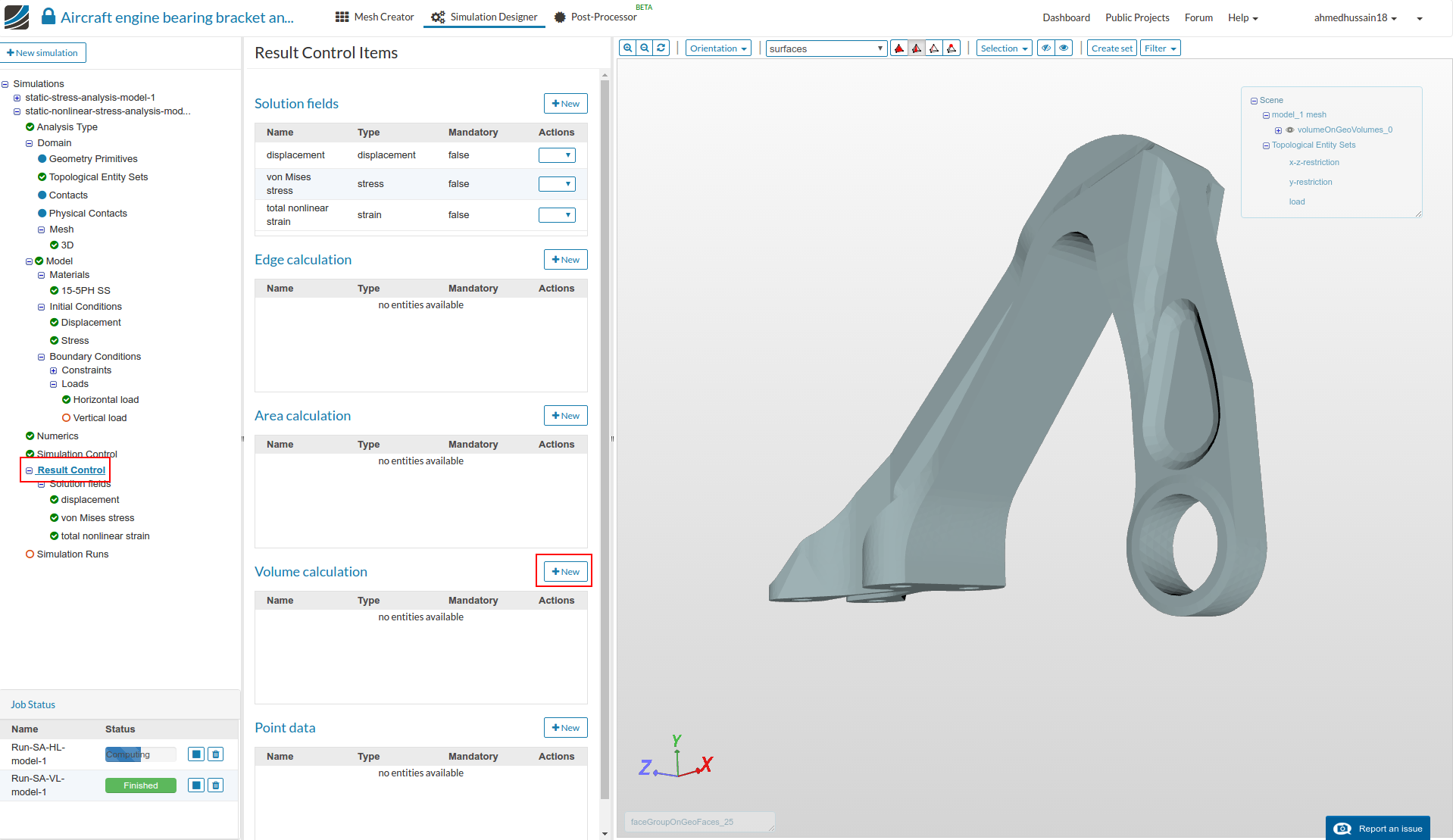
- Rename it to ‘vonMises stress in bearing bracket’ (optional), change ‘Field selection’ to stress and ‘Stress type’ to vonMises stress. Select the volume under ‘Topological Mapping’ and click ‘Save’ to save the changes.
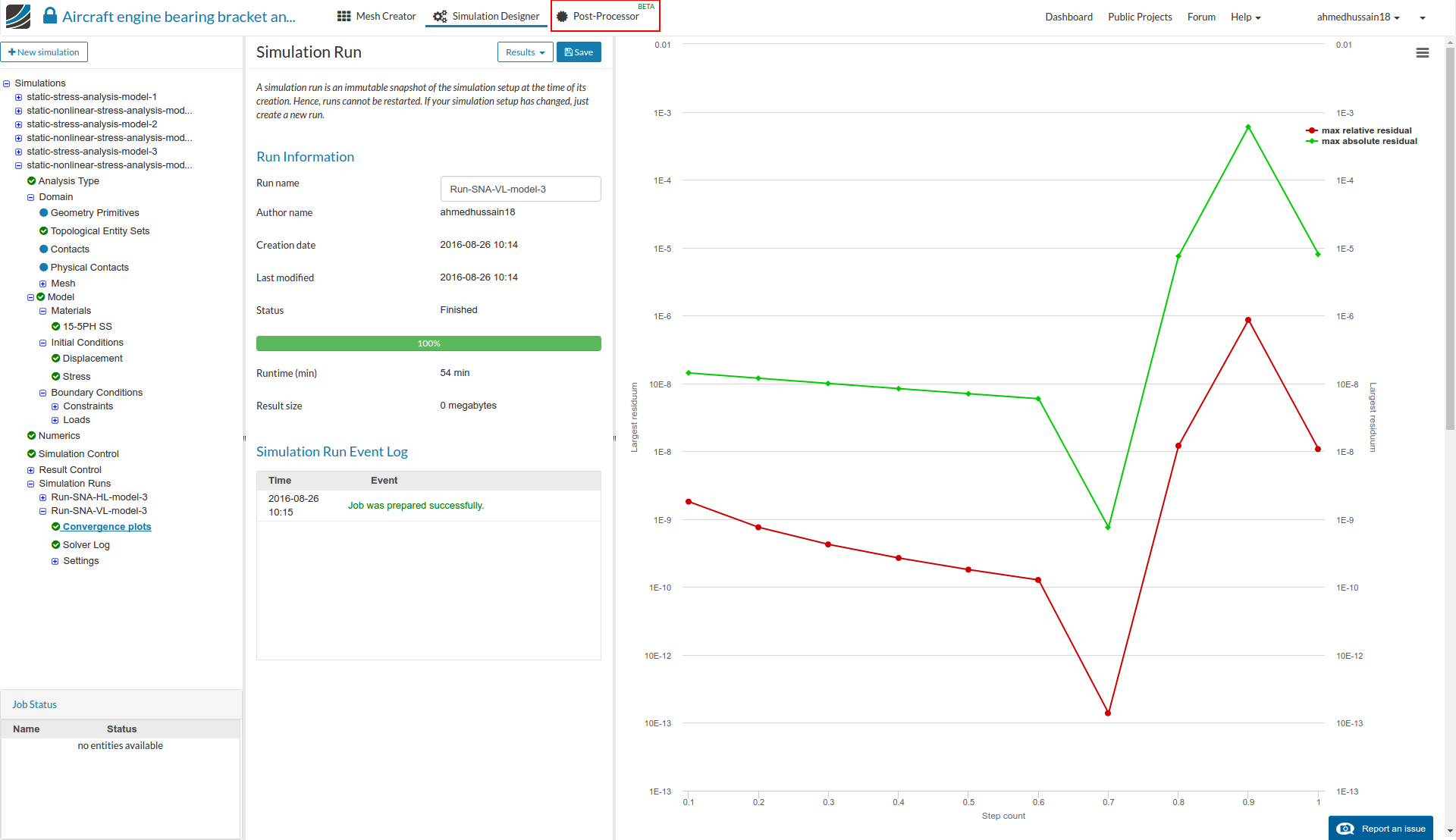
Simulation run
- That’s it for the nonlinear case. Create a new simulation run under ‘Simulation Runs’ and rename it to ‘Run-SNA-HL-model-1’ (optional) and click ‘Start’ to start the run.

- Simulation run will take approx. 30 min. to finish.
Vertical load case
- For applying the ‘Vertical load’ follow the same procedure as defined above.
Configuration 3:
-
For configuration 3, duplicate the first simulation i.e. ‘static-stress-analysis-model-1’ and rename it ‘static-stress-analysis-model-2’ (optional). Change the ‘Domain’ to model_2. Follow all the above steps in order to create topological sets and assign them back to boundary conditions. Make sure that you first assign ‘load’ set to ‘Horizontal load’ while un-assigning the ‘load’ from ‘Vertical load’.
-
Create a new run and rename it to ‘Run-SA-HL-model-2’ and click ‘Start’.
-
For ‘Vertical load’ case, please follow the above steps.
-
Create a new run and rename it to ‘Run-SA-VL-model-2’ and click ‘Start’.
Configuration 4:
-
For configuration 4, duplicate the second simulation i.e. ‘static-nonlinear-stress-analysis-model-1’ and rename it ‘static-nonlinear-stress-analysis-model-2’ (optional). Change the ‘Domain’ to model_2. Follow the above steps in order to assign the topological sets back to boundary conditions. Make sure that you first assign ‘load’ set to ‘Horizontal load’ while un-assigning the ‘load’ from ‘Vertical load’.
-
Please also make sure to assign volume to ‘vonMises stress in bearing bracket’ under ‘Result Control’.
-
Create a new run and rename it to ‘Run-SNA-HL-model-2’ and click ‘Start’.
-
For ‘Vertical load’ case, please follow the above steps.
-
Create a new run and rename it to ‘Run-SNA-VL-model-2’ and click ‘Start’.
Configuration 5 & 6:
- For configuration 5 and 6 do all the same as above by assigning the model_3 to ‘Domain’.
Post-processing
- Once all the simulations are over, click on Post-Processor tab to view the results.
Post-processing of linear case (Configuration 1, 3, 5):
-
First we will compare the results of the linear simulation cases. We will show here the post-processing of static analysis with horizontal load. Same procedure then can be used for post-processing of vertical load case.
-
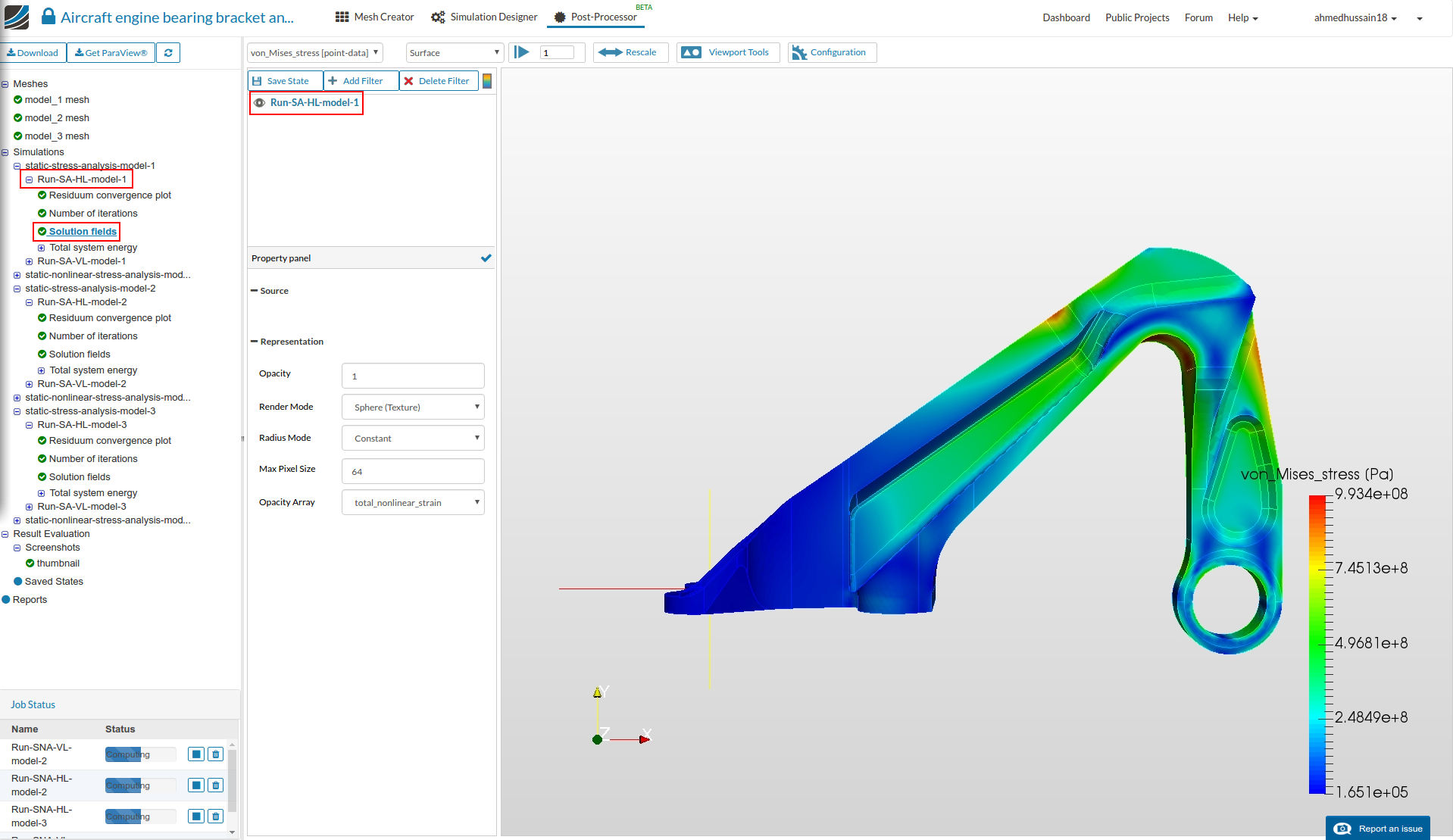
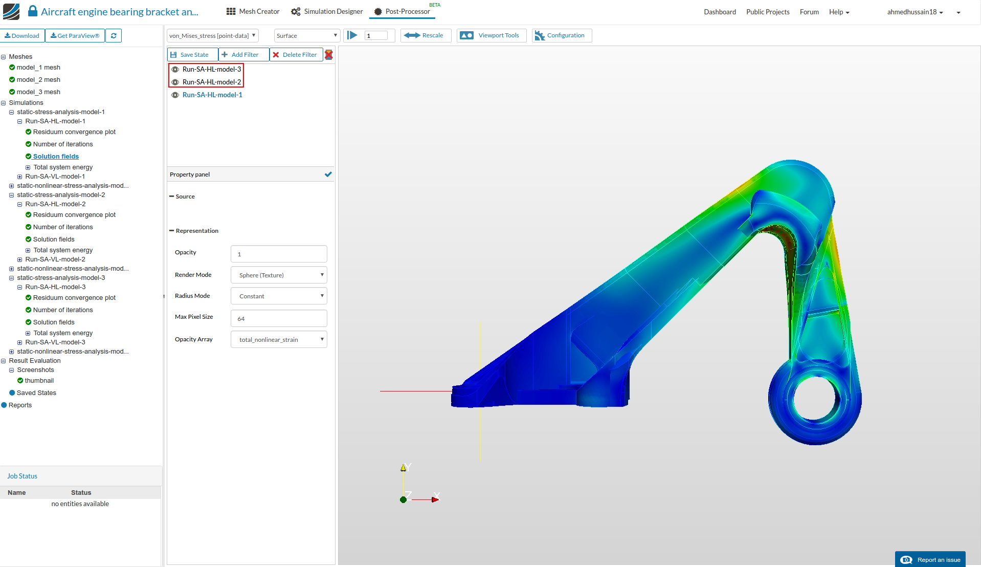
Select Solution fields of the simulation run of first model to view results i.e. Run-SA-HL-model-1. In a while the results will load in the viewer of post-processor.
- Next we will load the results of second model i.e. Run-SA-HL-model-2 in to the same viewer for comparison by clicking on it’s solution field and selecting Add result to viewer. This will load the results of second model in the same viewer.
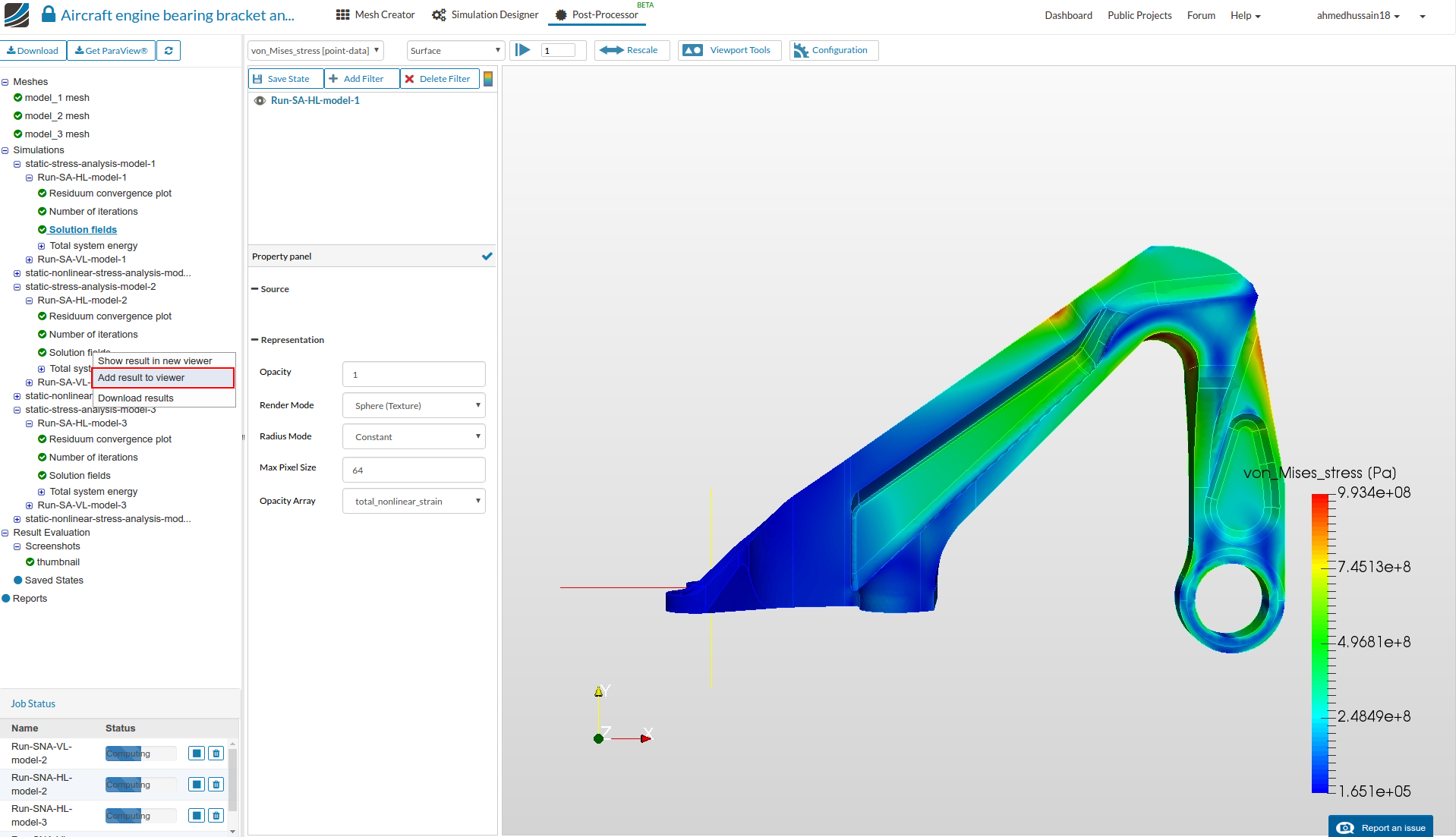
- Perform the same procedure to add the results of third model case i.e. Run-SA-HL-model-3 in this case.
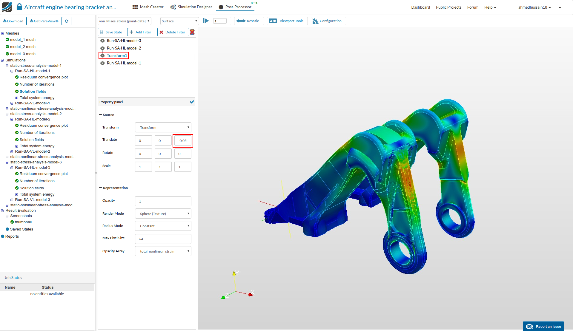
- Since all the models are overlapping, we will perform a transform operation in order to transform the models side-by-side in order to compare the results more easily. Click Run-SA-HL-model-2 and then click Add filter and select Transform filter. This will apply the transform filter to the selected solution field. Now change the Translate third column value to -0.05. This will transform the second model geometry by 0.05 meters in ‘-ve’ z-direction.
-
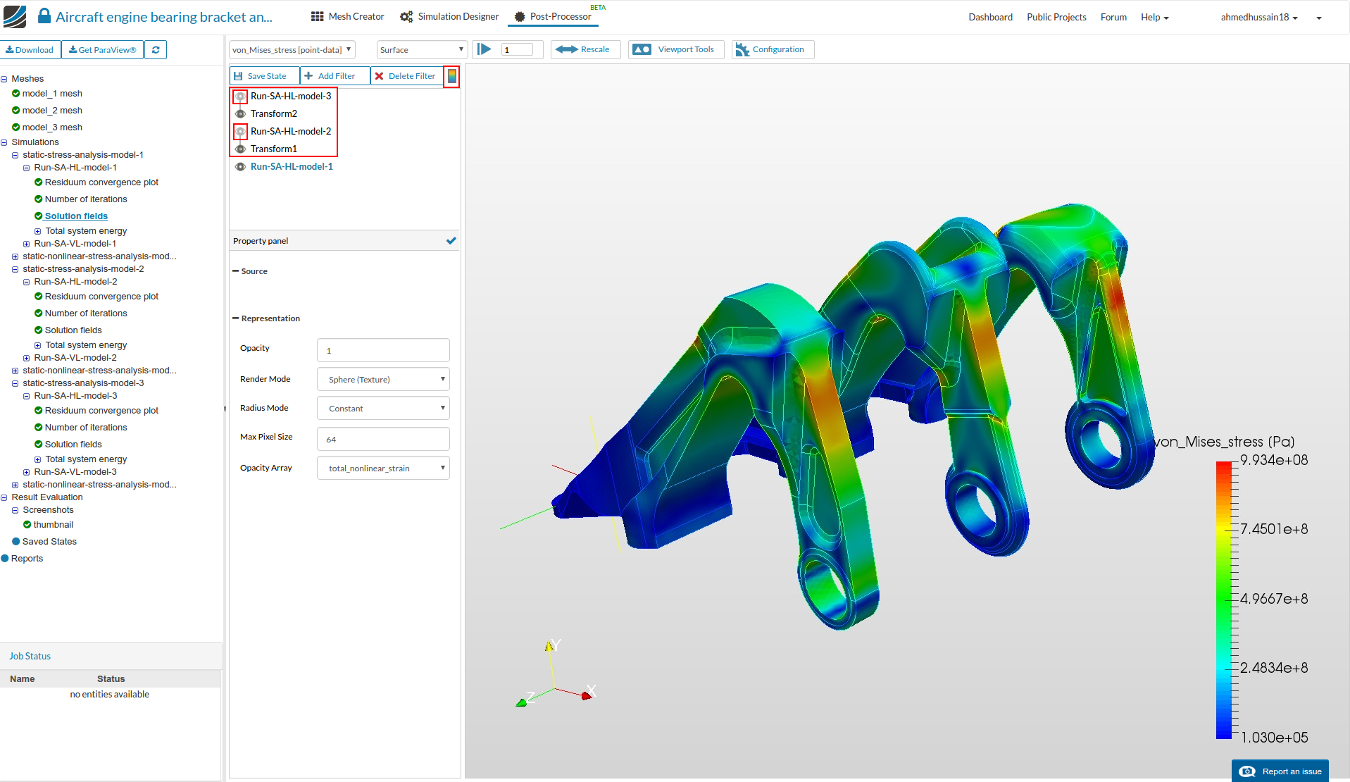
Perform the same operation for Run-SA-HL-model-3 but this time transform it by -0.1 by giving this value in third column next to Translate.
-
Furthermore, hide the other filters on which transform filter was applied by clicking the eye icon next to them. Then go back to Run-SA-HL-model-1 and toggle on the color bar by clicking the toggle bar button in middle top.
-
Next rescale the vonMises stress value from 0 to 1e9 (yield stress of 15-5PH SS) by going to Rescale option above. Click OK to save the changes. This will rescale the color bar for all the result cases.
-
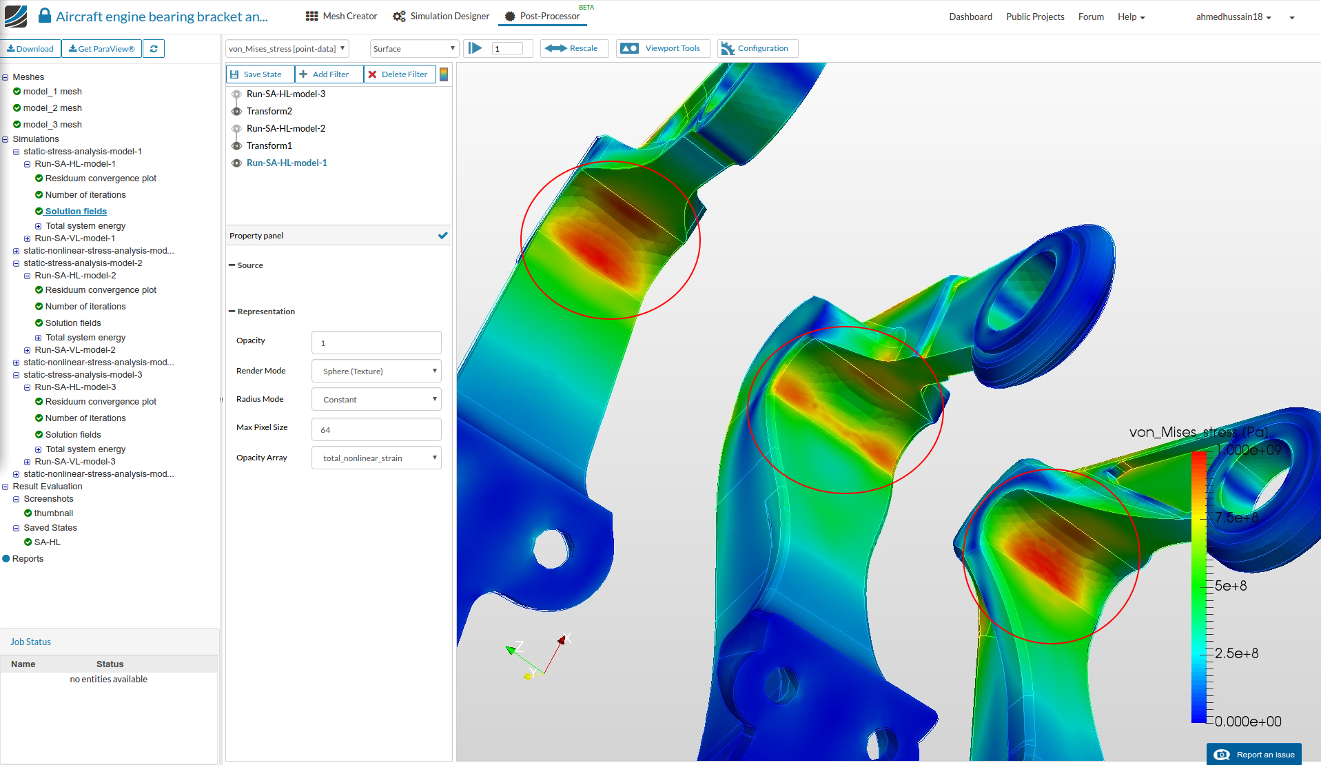
One can see that the stresses on the top front portion is more in the third model case which shows the early yielding of it at this load.

- Rotate the model and you will notice that first model as small high stress region in middle back due to sharp edge. Model 2 here is performing well as the load is distributed among the high raised portions. Third model has a quite nice distribution of stresses but it’s most of the area is stressed out from the back.
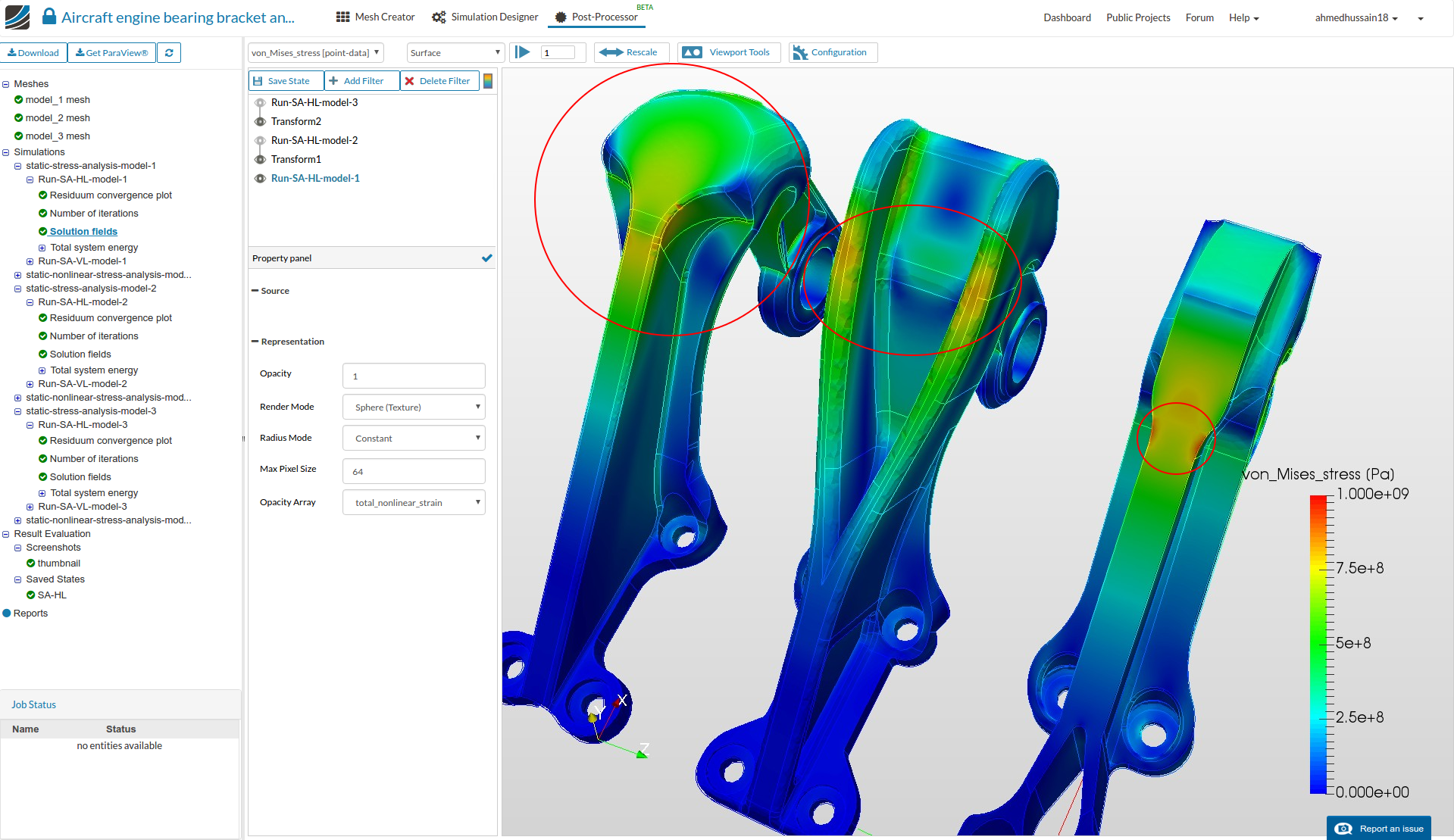
- Rotating it further to see the stresses in the interval curve one can reveal that first and third model has nearly same stress distribution on the curvature whereas, second model stresses are quite less leading which will lead to lesser yield area on higher loads.
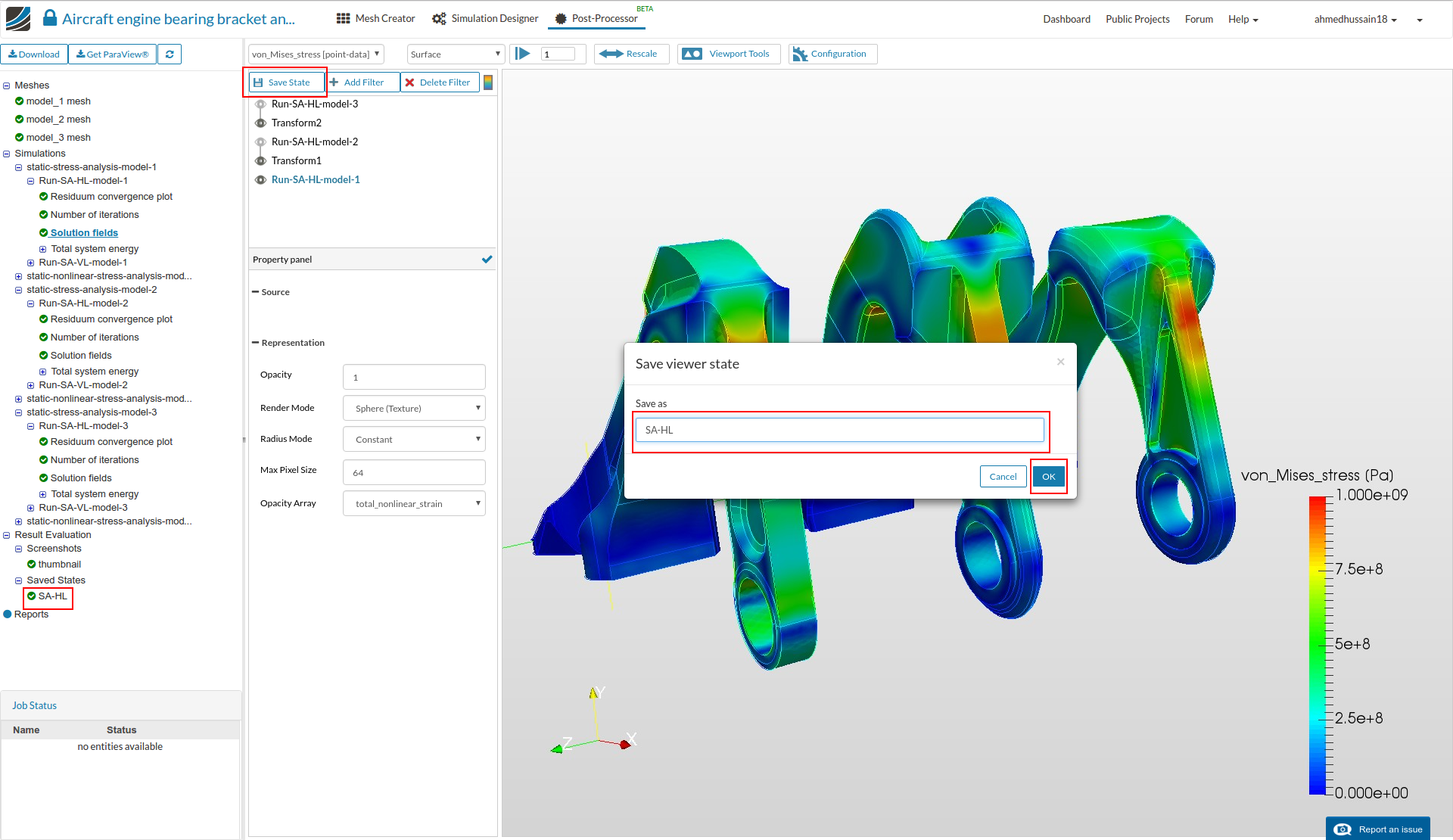
- You can now save the state for later use. Just click Save State and give it a reasonable name e.g. SA-HL in this case and click OK. You will see the your saved state under Saved State tree on the left.
- Now you can perform the same steps for the vertical load case.
Post-processing of nonlinear case (Configuration 2, 4, 6):
-
Now we will look in to the post-processing of the nonlinear case. We will do the post-processing of configuration 2, 4 and 6 with vertical load. Same steps can be followed to perform the post-processing for horizontal load case.
-
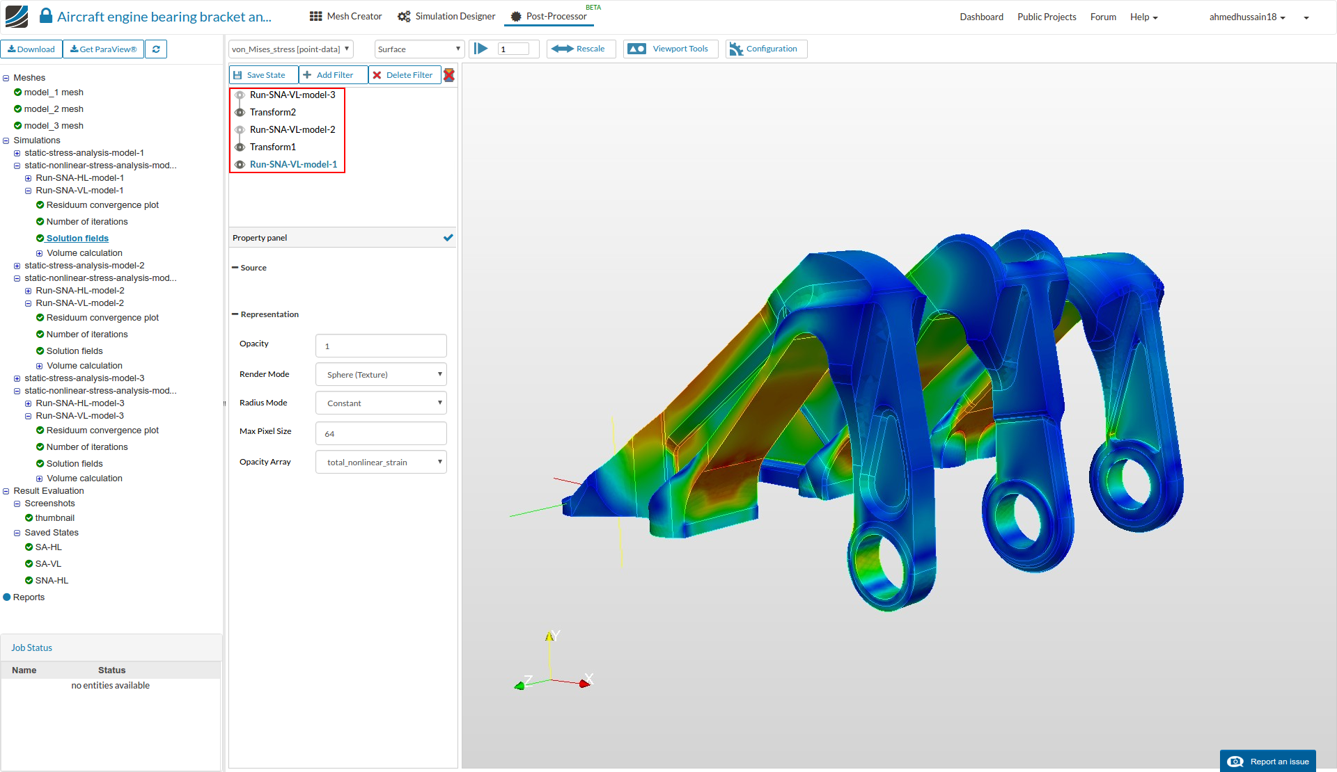
First of all do all the post-processing steps of linear case above with the results of nonlinear case i.e. Run-SNA-VL-model-1, Run-SNA-VL-model-2 and Run-SNA-VL-model-3.
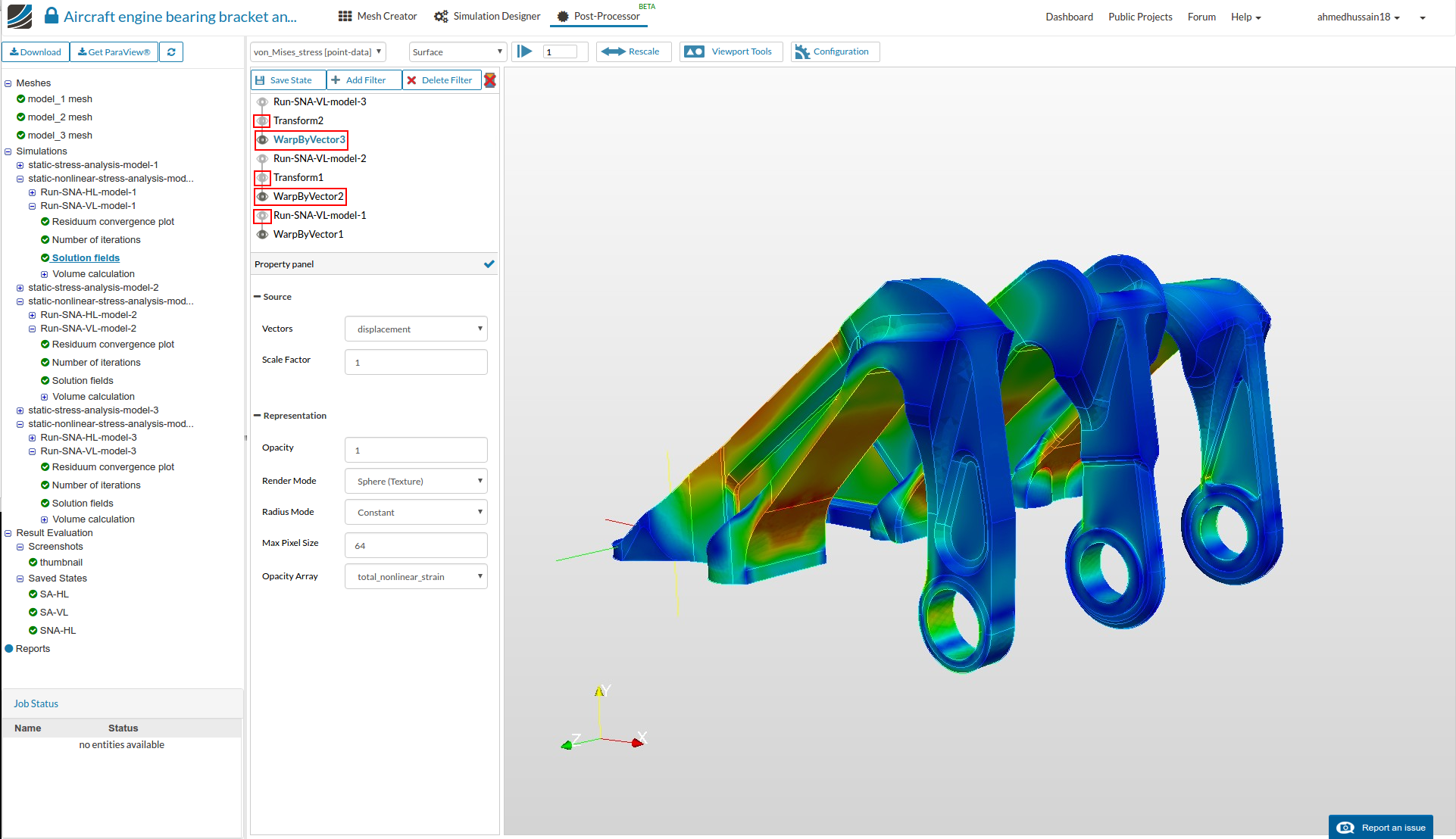
- Once you have get the same configuration of the results, proceed to apply a filter in order to get the deformed shapes of the geometry. Go to Run-SNA-VL-model-1 and then click Add Filter and select WarpByVector. This filter will show the deform state of the Run-SNA-VL-model-1 case.
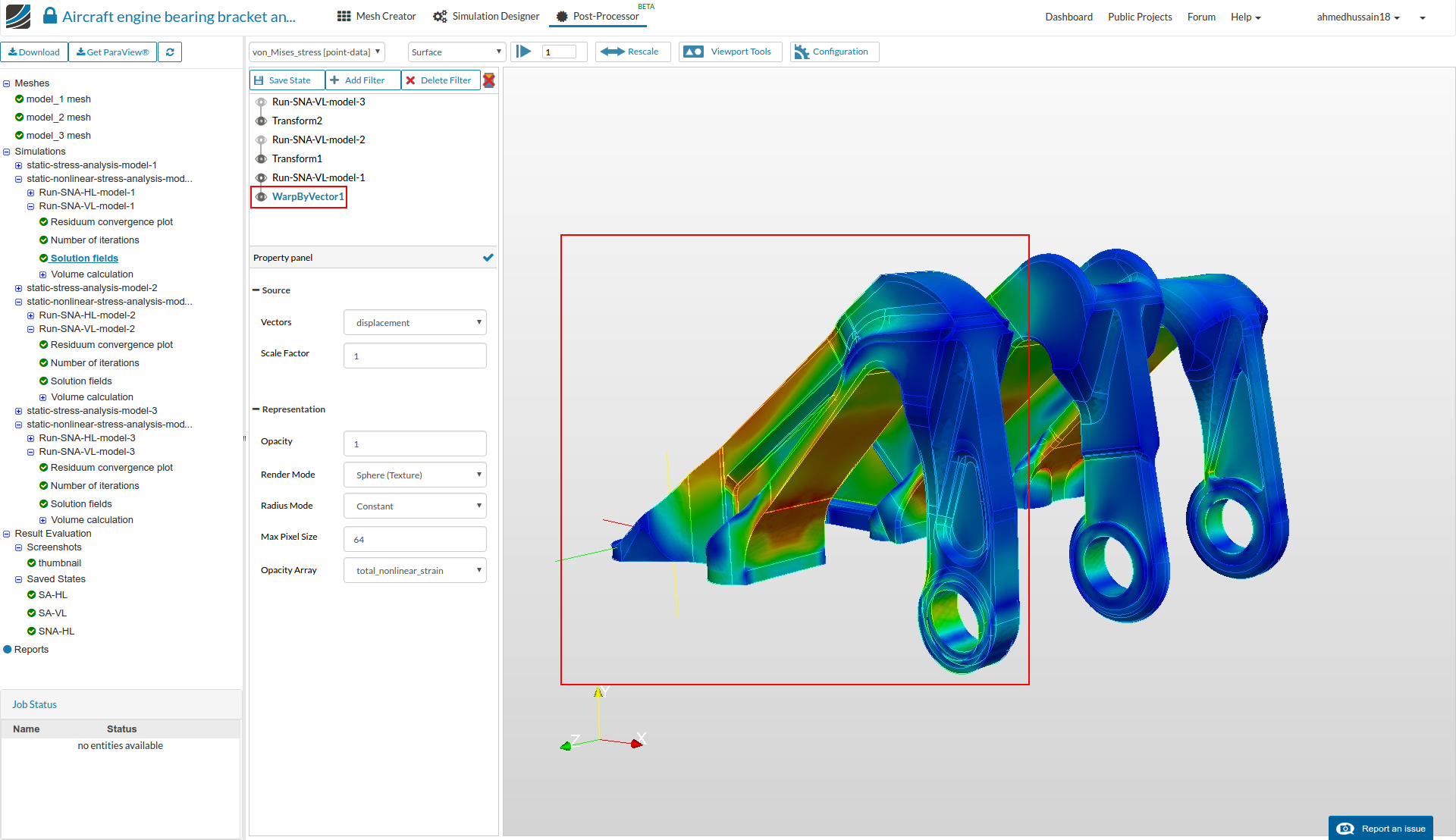
- Apply same filter to all transform filters of other models. Furthermore, hide all the solution fields to which this filter is applied by clicking the eye icon next to them. Your configuration should look something like this.
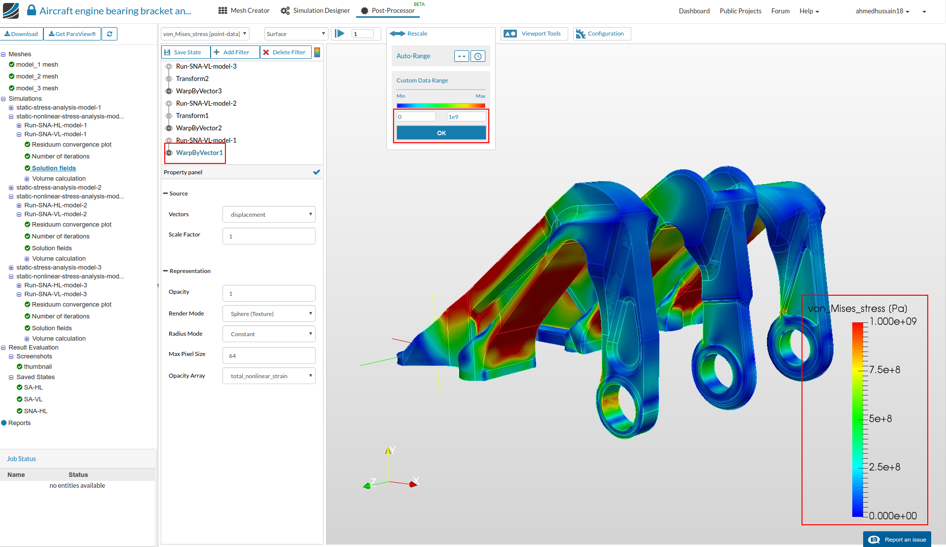
- Next go back to WarpByVector1 and rescale the vonMises stress from 0 to 1e9 (yield stress value of 15-5PH SS).
- Rotate the model to see the internal side of the bearing brackets. One can see the the first model is yielded the most (represented by the red region) compared to other two models.
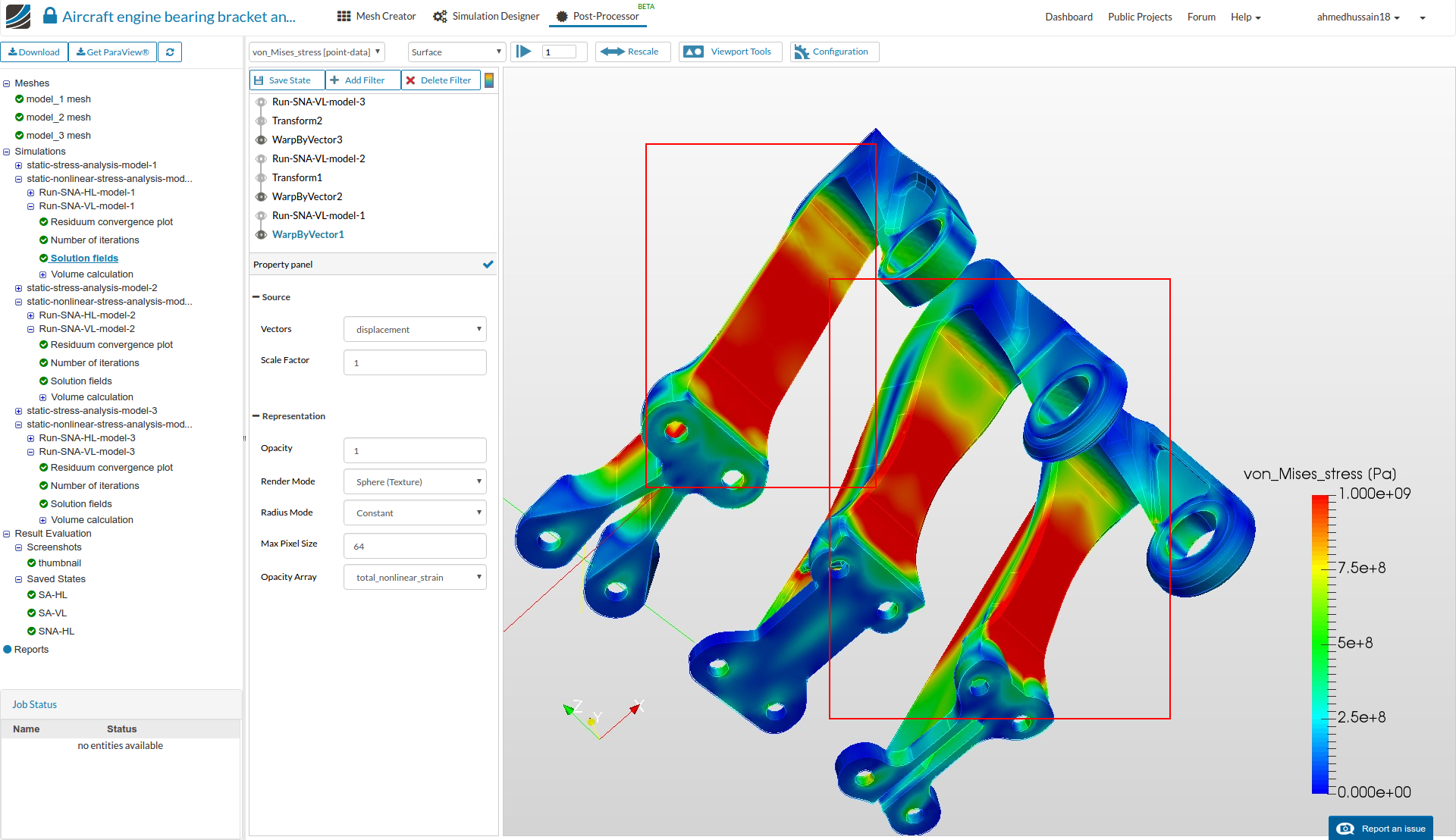
- Looking at the back of the models one can again see highly yielded first compared compared to others. Whereas, second model stresses are distributed well between two elevated regions making the internal extrusion yielded very slightly. The third model compared to others is yielded fairly less.
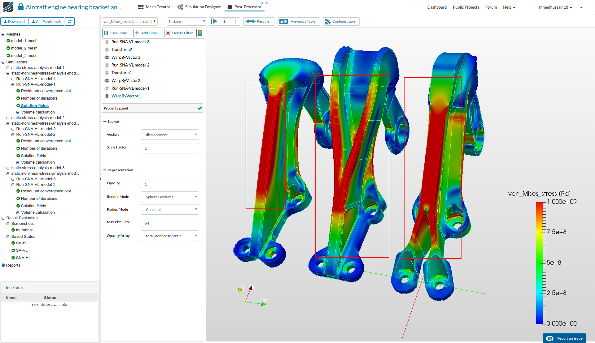
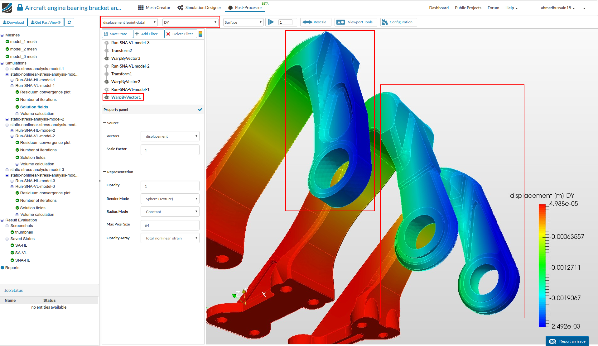
- Next up we will look in to the y-displacement of the models. For this change the Array name to displacement [point-data] and then Array component to DY. Do this for all the WarpByVector filters and then rescale it according to WarpByVector1. One can then see that the first model is more displaced compared to other models. The reason behind this can be a thinner form of the model compared to others.
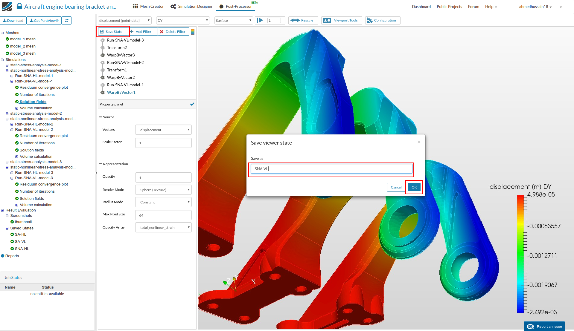
- You can now save the state for later use. Just click Save State and give it a reasonable name e.g. SNA-VL in this case and click OK. You will see the your saved state under Saved State tree on the left.
- Now you can perform the same steps for the horizontal load case.
Conclusion
-
All the three models are well designed bearing easily reasonable amount of load. But according to our test we can conclude the following points:
-
Though having a good strength/mass ratio (please see the start of the homework), model_1 is fairly easy to get yielded compared to other models.
-
Also due to less weight and thin structure, model_1 is easily bendable compared to other models.
-
According to our testing, the second model gives fairly nice combination of strength with considerably increased weight. But overall the performance of model_2 is better than the others thanks to the wide structure and two extruded portions on the back.
-
References:
[1] Spierings, A. B., T. L. Starr, and K. Wegener. “Fatigue performance of additive manufactured metallic parts.” Rapid Prototyping Journal 19.2 (2013): 88-94.
