# What is y+ (yplus)?
**URL:** https://www.simscale.com/forum/t/what-is-y-yplus/82394
**Category:** Fluid Flow / CFD
**Created:** [May 1, 2018, 10:37am UTC](https://www.simscale.com/forum/t/what-is-y-yplus/82394 "2018-05-01T10:37:49Z")
**Posts on this page:** 3
**Page:** 1
### Author:  [@jousefm](https://www.simscale.com/forum/u/jousefm)
#### Post date: [May 1, 2018, 10:37am UTC](https://www.simscale.com/forum/t/what-is-y-yplus/82394/1 "2018-05-01T10:37:49Z")
**There can never be a last word in regard to the axioms of any physical theory. All we can ask of them is that they lead to conclusions in agreement with observation. Sooner or later more refined observations will find the weak point in any set of physical axioms. Nature is far too complicated to be completely described in a few equations.** - J.L. Synge (1938)
* * *
\underline{\textbf{Introduction}}
Before World War II, Johann Nikuradse (known from the Nikuradse Diagram) took a bunch of velocity measurements in smooth pipes at different distances from the inside wall surface and, in 1933, **[published](https://ntrs.nasa.gov/archive/nasa/casi.ntrs.nasa.gov/19930093938.pdf)** his results with the title “ **Strömungsgesetze in rauhen Rohren** ” (“Laws of flow in rough pipes”). The first empirical friction law has already been proposed by Chézy in 1775 ^1, when this engineer had to determine the cross section of channels necessary to provide water to the city of Paris. In the 1860s, another French engineer called Bazin had taken measurements of velocity in rectangular and trapezoidal flumes, resulting in a huge amount of data sets. A big problem here was the trend lines didn’t match, although each set showed a relationship between velocity and wall distance. Nobody could write an equation to describe exactly how velocity behaves from the near wall region or far away from the wall until Nikuradse and his teacher, Prandtl, **normalized** the axes into **y^+** (the axis that used to be the distance) and **u^+** (the axis that used to be velocity). The result was that all the data sets perfectly matched. In addition, the two engineers could also write an equation that would fit u+ and y+ near the wall!
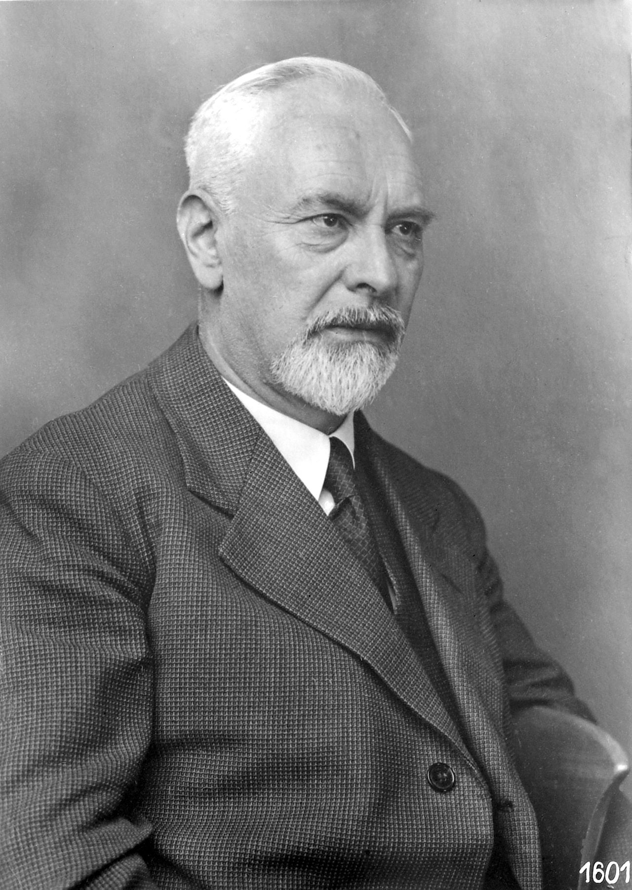
**Figure 1:** German engineer Ludwig Prandtl
In **[CFD (Computational Fluid Dynamics)](https://www.simscale.com/docs/content/simwiki/cfd.html)**, that equation is still used as a function to figure out the shear stress at a wall node. In this SimWiki post, we are going to cover the fundamentals of y^+ as well as u^+, why they are used and why these values are very important!
\underline{\textbf{Why using wall functions?}}
Turbulent flows are an omnipresent phenomenon in **[CFD (Computational Fluid Dynamics)](https://www.simscale.com/docs/content/simwiki/cfd.html)** and are significantly affected by the presence of walls, where the viscosity-affected regions have large gradients in the solution variables. An accurate representation of the near wall region determines a **successful prediction of wall bounded turbulent flows**.
Some mature turbulence models such as k-\epsilon are only valid in the **area of turbulence fully developed** , and do not perform well in the area close to the wall. In order to deal with the near wall region, **two ways** are usually proposed.
1. One way is to integrate the turbulence to the wall. Turbulence models are modified to enable the viscosity-affected region to be **resolved with all the mesh down to the wall** , **including the viscous sublayer**. When using a modified low Reynolds turbulence model to solve the near-wall region, the first cell center must be placed in the viscous sublayer (preferably y^+ = 1) leading to the requirement of abundant mesh cells. Thus, substantial computational resources are required.
* * *
1. Another way is to use the so-called **wall functions** , which can **model the near wall region**. Wall functions are equations empirically derived and used to **satisfy the physics** in the near wall region. The **first cell center** needs to be placed in the **log-law region** to ensure the **accuracy** of the results. Wall functions are used to **bridge** the inner region between the wall and the turbulence fully developed region. When using the wall functions approach, there is **no need to resolve the boundary layer** causing a significant **reduction of the mesh size and the computational domain**!
* * *
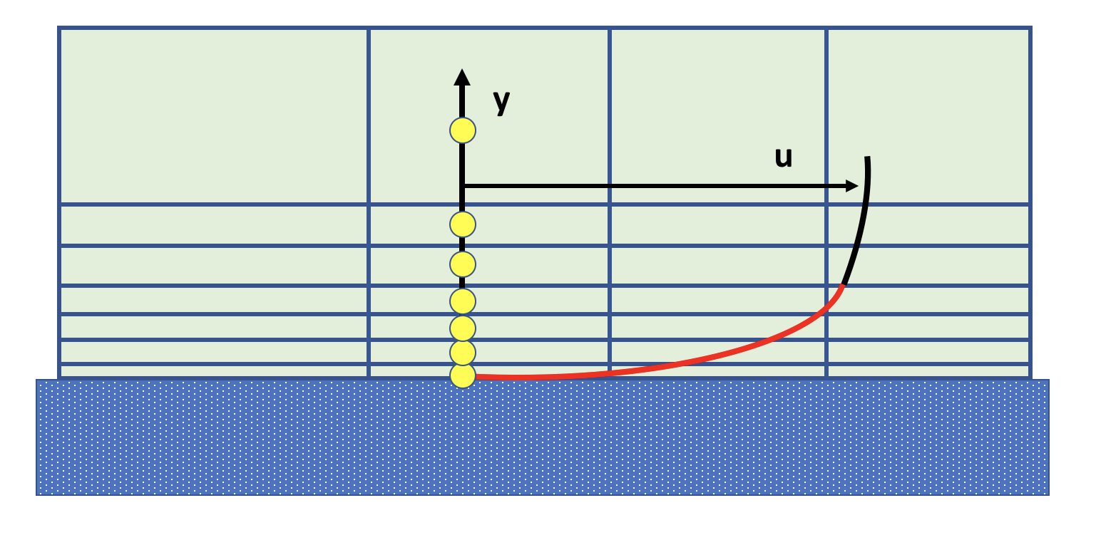
**Figure 2:** Viscous sublayer resolving approach to resolve boundary layer (in red)
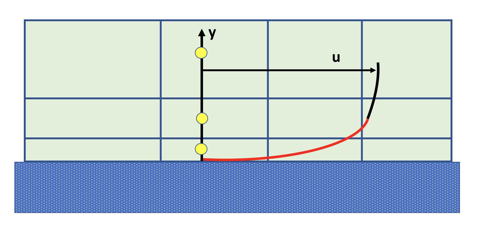
**Figure 3:** Logarithmic-based Wall functions to resolve boundary layer (in red)
* * *
\underline{\textbf{Wall functions}}
“_ **At a high Reynolds number, the viscous sublayer of a boundary layer is so thin that it is difficult to use enough grid points to resolve it** _” (Ferziger and Perić 2002).
The wall functions rely on the **universal law of the wall** , which basically states that the velocity distribution very near to a wall is similar for almost all turbulent flows. One of the most prominent parameters when judging the applicability of wall functions is the so-called dimensionless wall distance y^+ (Schlichting and Gersten 2001) denoted by:
y^+ = \frac{y u\_\tau}{\nu} \tag{1}
1. u\_\tau is the so called **friction velocity**
2. y is the **absolute distance** from the wall
3. \nu is the **kinematic viscosity**
One can interpret y^+ as a local Reynolds number, which means that its magnitude can be expected to determine the relative importance of viscous and turbulent processes. Figure 2 shows the fractional contributions to the total stress from the **viscous** and **Reynolds stresses** in the near wall region of channel flow. (Pope)
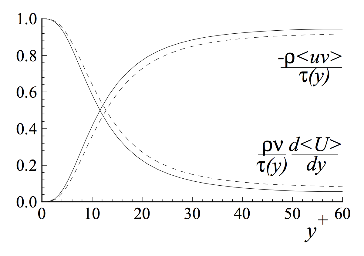
**Figure 4:** Profiles of fractional contributions of the viscous and Reynolds stresses to the total stress. DNS data of Kim _et al._ (1987): dashed lines, Re = 5,600; solid lines, Re = 13,750.
One can easily see that if we are in the **viscous wall region** with y^+ \< 50, there is a direct effect of the viscosity on the shear stress. Conversely in the **outer layer** with y^+ \> 50, the effect of viscosity is neglibile.
For the sake of completeness, let’s briefly introduce the **friction velocity** u\_\tau. It should be evident that the viscosity \nu and wall shear stress \tau\_w are important parameters. From these quantities and \rho we define the **viscous scales** being appropriate viscous scales and lengthscales in the near-wall region.
u\_\tau = \sqrt{\frac{\tau\_w}{\rho}} \tag{2}
with
\tau\_w = \rho \nu \left(\frac{d\}{dy} \right)\_{y = 0} \tag{3}
The dimensionless velocity is given by:
u^+= \frac{u}{u\_\tau} \tag{4}
* * *
Stephen B. Pope (2000) comments on the steep velocity profile near the wall and how turbulence model needs to take this into account. This is also the point where wall functions come into play, first suggested by B.E. Launder and Spalding (1972). The basic idea is that additional boundary conditions are applied at some distance to the wall to fulfill the **log-law**. Hence the additional equations introduced by the turbulence model are not solved close to the wall. Depending on the turbulence model used, different wall functions must be applied to respective fields of the turbulence model, which means that k-\epsilon has different wall functions than the k-\omega model.
Due to this fact, the different turbulence models and the associated wall functions require different values of y^+ as well as different spatial resolutions of the near wall area. Please note that if the **log-law** region is **resolved geometrically** **by the mesh** , **no wall functions must be applied**! The downside of this approach is that depending on the simulation, such low y^+ values are **hard to create** during the pre-processing step (meshing) or even **undesirable** , as this will **significantly decrease the time step**!
In SimScale (using OpenFOAM as its CFD solver), **[wall functions](https://www.simscale.com/docs/content/simulation/model/boundaryConditionTypes/OF_new_wall.html?highlight=wall%20function)** are nothing else than boundary conditions that are applied to boundary patches of type **wall** , rather then a usual **patch**.
* * *
\underline{\textbf{Wall Regions and Layers as well as their Properties}}
1. **The viscous sublayer (y^+ \< 5)**
In the viscous layer, the fluid is dominated by the viscous effect, so it can be assumed that the Reynolds shear stress is negligible. The “linear velocity law” is given by:
u^+ = y^+ \tag{5}
1. **The logarithmic area (y^+ \> 30)**
In the logarithmic layer, turbulence stress dominate the flow and velocity profile varies very
slowly with a logarithmic function along the distance y. Formula (6) describes this region with the Karman constant \kappa of 0.41 and the constant B = 5.2.
u^+ = \frac{1}{\kappa} ln(y^+) + B \tag{6}
1. **The Buffer layer (5 \< y^+ \< 30)**
The **buffer layer** is the transition region between the viscosity-dominated region and turbulence-dominated part of the flow. Viscous and turbulent stresses are of **similar magnitude** and since it is complex, the velocity profile is not well defined and the original wall functions avoid the first cell center located in this region.
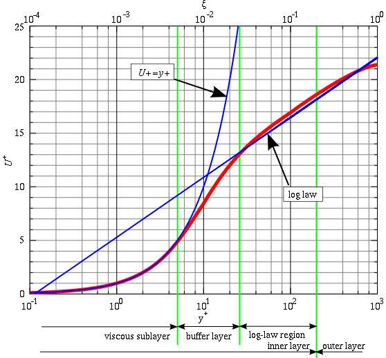
**Figure 5:** The Law of the Wall
* * *
\underline{\textbf{Best Practices}}^2
- In the pre-processing stage of the simulation we need to make sure that y^+ is in the desired range. For that, we have to calculate the size of the first layer of our mesh.
- Check the y^+ value after the computation again as the real flow field will develop during the simulation and a remesh might be necessary.
* * *
\underline{\textbf{Step-by-Step: Calculating Wall distance with a given y+}}
1. **Write down definition of y^+ and rearrange for y**
y^+ = \frac{y u\_\tau}{\nu} \space \rightarrow \space y = \frac{y^+ \nu}{u\_\tau} \tag{7}
1. **Next, we calculate u\_\tau**
u\_\tau = \sqrt{\frac{\tau\_w}{\rho}} \tag{8}
1. **The wall shear stress \tau\_w can be calculated from the skin friction coefficient C\_f**
\tau\_w = \frac{1}{2} C\_f \rho U^2\_\infty \tag{9}
1. **Determine the skin friction coefficient (for example, for a flat plate with the 1/7 power law)**
C\_f = 0.0576 Re\_d^{-\frac{1}{5}} \tag{10}
1. **The Reynolds number is known. Insert that into formula (10), the result in formula (9) and this into (8)**
2. **Now insert everything into formula (7) with your wanted y^+ and you are finished!**
* * *
Alternatively use a y^+ calculator: **[Y+ Calculator - Instantly Calculate First Wall Distance for CFD](https://www.simscale.com/blog/y-plus-calculator/)**
A list of skin friction coefficients can be found here: **[Skin friction coefficient -- CFD-Wiki, the free CFD reference](https://www.cfd-online.com/Wiki/Skin_friction_coefficient)**
* * *
\underline{\textbf{Limitations of Wall Functions}}^2
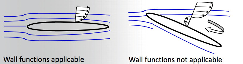
**Figure 6:** Wall functions and their limits
In the case of a boundary layer separation as depicted above, one should not use wall functions because the log-based wall functions do not correctly predict the profile. One should directly resolve the viscous sublayer to obtain accurate results.
* * *
\underline{\textbf{Other options for Wall Modelling}}^3
- **Enhanced Wall Treatment Option**
- **Scalable Wall Functions**
* * *
\underline{\textbf{Project Example}}
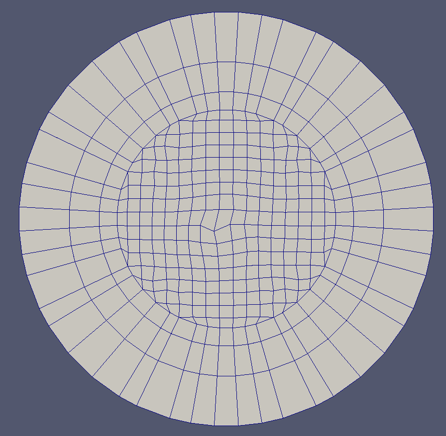 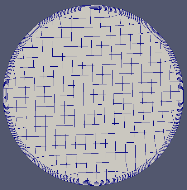
**Figure 7:** Meshes used for the Turbulent Pipe Flow validation: left is used for wall function (y^+ ≈ 30) approach, right for full resolution (y^+ ≈ 1) approach.
This validation case can be found here: **[Turbulent Pipe Flow Validation](https://www.simscale.com/docs/content/validation/TurbulentPipeFlow/TurbulentPipeFlow.html)**
* * *
\underline{\textbf{Y+ (yplus) - Generate Wall Spacing for CFD on SimScale}}
The following page explains how you can generate the desired y+ (yplus) value on SimScale and check if your settings are correct: **[Y+ (yplus) - Generate Wall Spacing for CFD](https://www.simscale.com/forum/t/y-yplus-generate-wall-spacing-for-cfd/82451)**
* * *
\underline{\textbf{Literature}}:
- **F. Liu - A Thorough Description Of How Wall Functions Are Implemented In OpenFOAM**
- **S. M. Salim, S.C. Cheah - Wall y^+ Strategy for Dealing with Wall-bounded Turbulent Flows**
- **T. Marić, J. Höpken, K. Mooney - The OpenFOAM Technology Primer**
- **Stephen B. Pope - Turbulent Flows**
* * *
\underline{\textbf{References}}:
[1] - **A. Chezy - Formule pour trouver la vitesse de l’eau conduite dans une rigole donnée**
[2] - **[Turbulence Fluent Notes](https://www.researchgate.net/profile/Panayampilly_Abdul_Samad/post/y_plus_range_for_turbulent_models/attachment/59d6393c79197b8077996735/AS%3A400990483304449%401472614989133/download/Fluent-Intro_15.0_L07_Turbulence.pdf)**
[3] - **[Fluid Lecture 06 Turbulence](http://imechanica.org/files/fluent_13.0_lecture06-turbulence.pdf)**
* * *
\underline{\textbf{Pictures}}:
- **Figure 1:** **[Ludwig Prandtl - Wikipedia](https://en.wikipedia.org/wiki/Ludwig_Prandtl)**
- **Figure 2:** Created with PowerPoint
- **Figure 3:** Created with PowerPoint
- **Figure 4:** **[https://pope.mae.cornell.edu/TurbulentFlows/popefigures/pdf/chapter7Figures.pdf](https://pope.mae.cornell.edu/TurbulentFlows/popefigures/pdf/chapter7Figures.pdf)**
- **Figure 5:** **[https://en.wikipedia.org/wiki/Law\_of\_the\_wall](https://en.wikipedia.org/wiki/Law_of_the_wall)**
- **Figure 6:** **[Turbulence Fluent Notes](https://www.researchgate.net/profile/Panayampilly_Abdul_Samad/post/y_plus_range_for_turbulent_models/attachment/59d6393c79197b8077996735/AS%3A400990483304449%401472614989133/download/Fluent-Intro_15.0_L07_Turbulence.pdf)**
- **Figure 7:** SimScale Documentation
* * *
\underline{\textbf{Acknowledgement}}:
I am deeply grateful to Barry (@Get_Barried), Darren (@1318980), as well as Jozsef Nagy for proofreading and making suggestions to make sure users can get most out of this SimWiki article.
---
### Author:  [@Get\_Barried](https://www.simscale.com/forum/u/Get_Barried)
#### Post date: [May 1, 2018, 10:41am UTC](https://www.simscale.com/forum/t/what-is-y-yplus/82394/2 "2018-05-01T10:41:23Z")
Brilliant work @jousefm! Looking forward to more!
---
### Author:  [@jousefm](https://www.simscale.com/forum/u/jousefm)
#### Post date: [August 5, 2018, 9:01am UTC](https://www.simscale.com/forum/t/what-is-y-yplus/82394/3 "2018-08-05T09:01:17Z")