Recording
Homework Submission
For your homework, your task is to simulate the blood flow through 3 different arteries, the first, with a healthy blood vessel with no calcification or blockage; the second, through a moderately calcified blood vessel and the third, through a severely calcified or occluded blood vessel.
The step-by-step tutorial below contains all of the steps for setting up the simulation in SimScale and visualizing the results.
To submit your homework assignment, please generate a public link of your project (Sharing a Project)
Homework Deadline: Sunday, February 18th, 11:59 pm CET
Submit your homework here
Introduction
In this exercise, we will focus on simulating the flow of blood as a non-newtonian fluid through a Carotid Artery Bifurcation. The simulations are performed for 3 cases - the first, with a healthy blood vessel with no calcification or blockage; the second, through a moderately calcified blood vessel and the third, through a severely calcified or occluded blood vessel. The results will show the differences in pressure, velocity profile, and the outlet flow through the 2 branches.
The image below shows an overview of the 3 different cases:
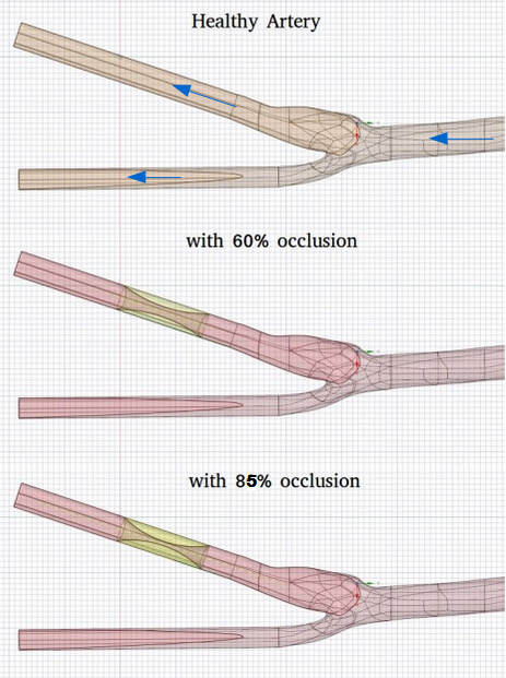
This tutorial presents a step by step approach for simulating the third case with 85% occlusion of the Artery. The first 2 cases can then be done by duplicating the setups and following similar steps.
Import Project
To start this exercise, please import the project into your workspace by clicking on the link below:
Mesh Generation
In the Mesh Creator tab, click on the geometry Case -3-85-pc-blocked
Then, click on the New Mesh button in the options panel.
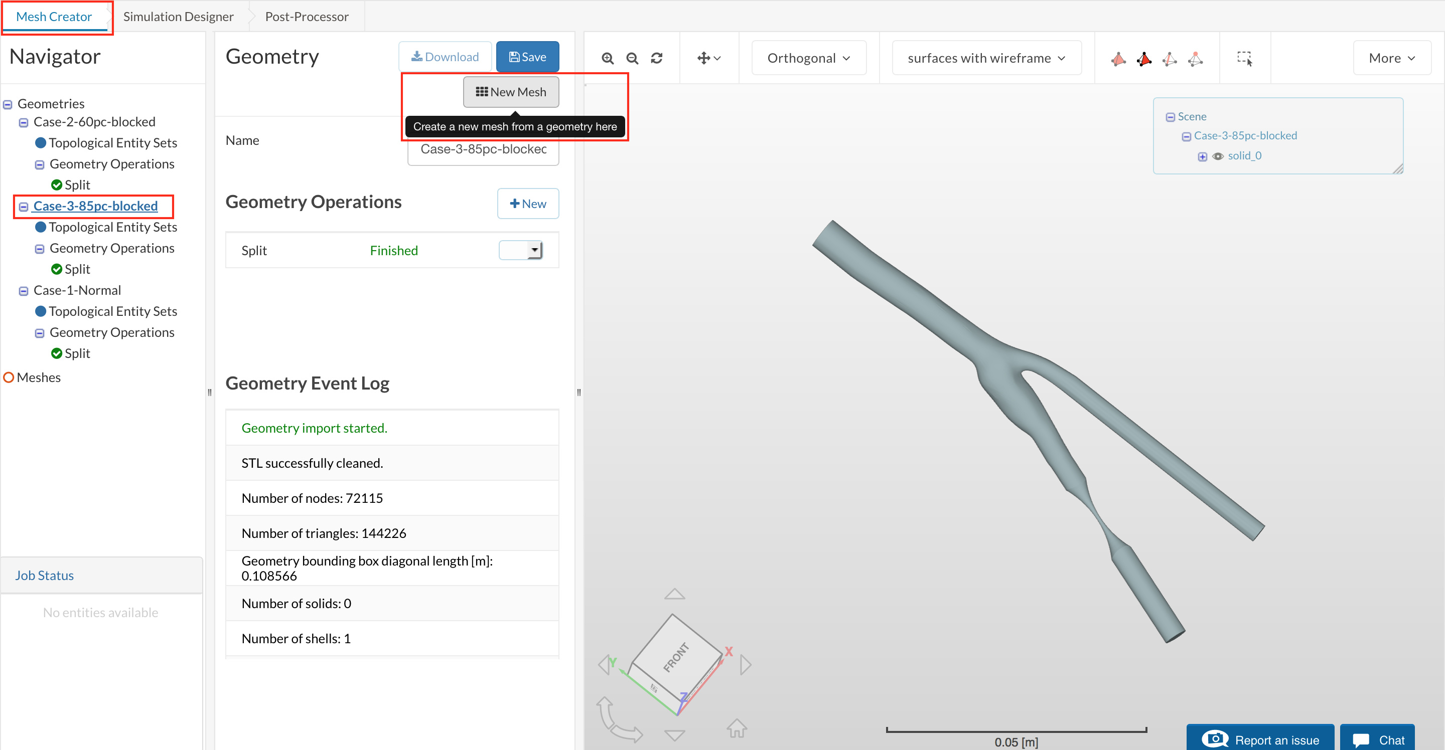
Figure 2: Creating a new mesh from geometry
Select the mesh Type Hex-dominant parametric. Then specify the following parameters:
- Number of cells in X-direction: 45
- Number of cells in Y-direction: 150
- Number of cells in Z-direction: 20
- Number of computing cores: 16
Click Save to preserve the mesh settings
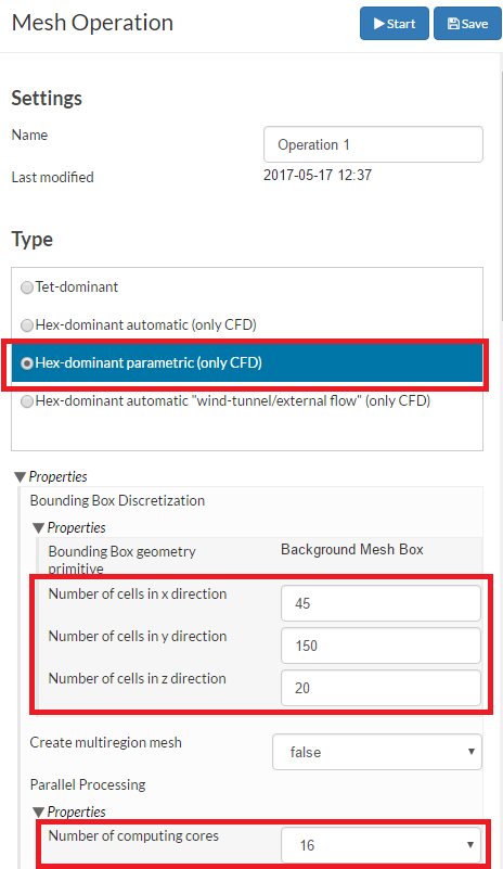
Figure 3: Base mesh cells and number of core selection.
After saving the Navigator is expanded with 2 new entries, called Background Mesh Box and Material Point which must be defined.
The Background Mesh Box defines the reference bounds of the base mesh. Enter the values as shown or use the default values:
- Min X= -0.019
- Min Y= -0.065
- Min Z= -0.004
- Max X= 0.013
- Max Y= 0.0415
- Max Z= 0.01
Click Save to preserve the mesh settings
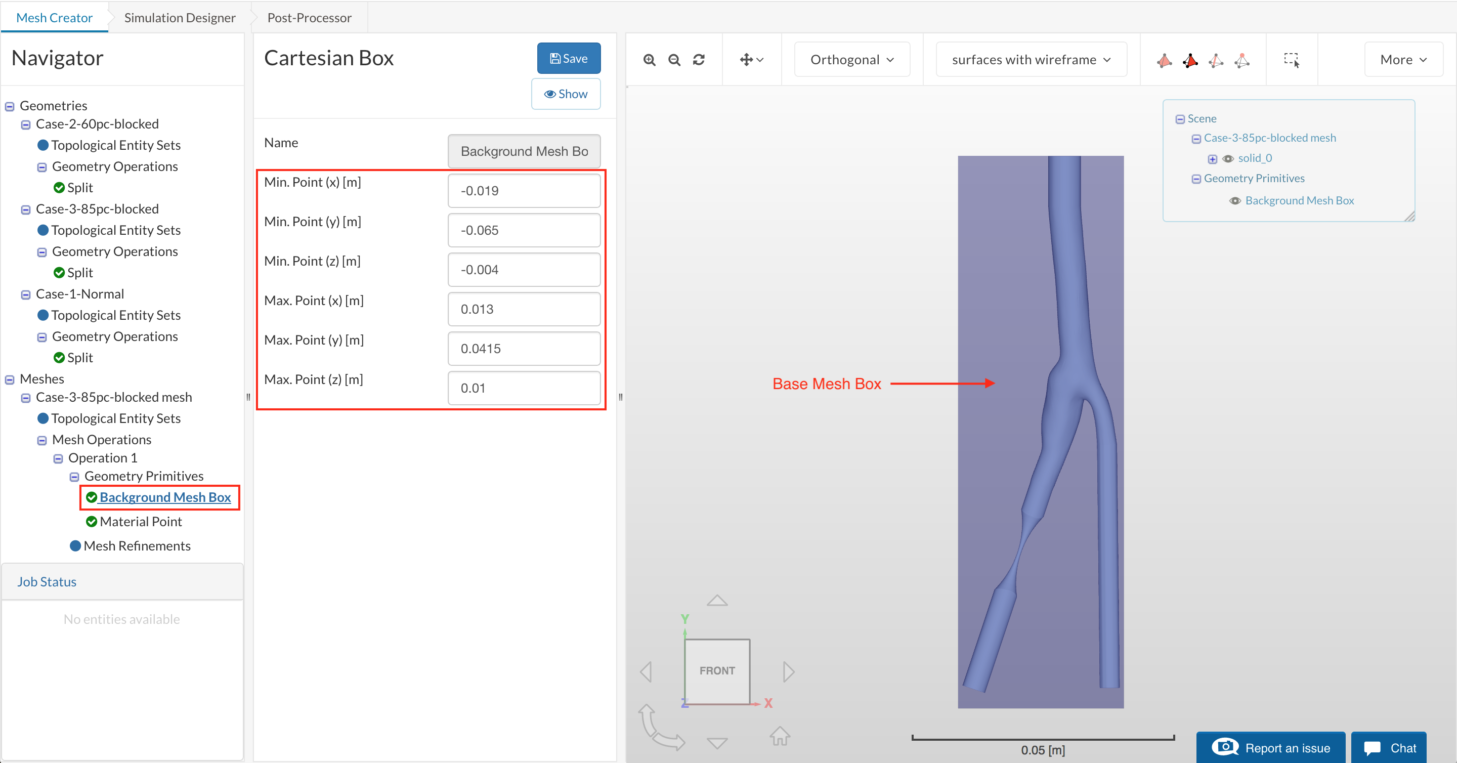
Figure 4: Background Mesh Box settings.
The Material Point specifies the region that will be meshed. So, in this case, the point must be inside the body.
Enter the values:
- Center X= 0.0025
- Center Y= 0.001
- Center Z= 0.0025
Click Save to preserve the mesh settings
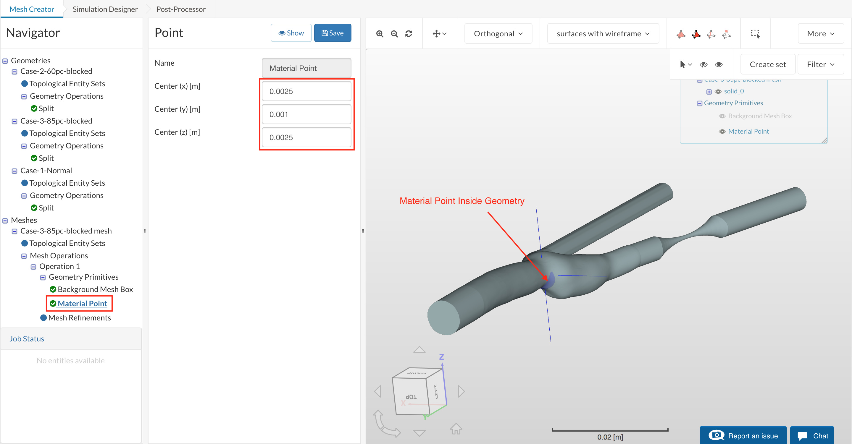
Figure 5: Material point located inside the geometry to ensure internal mesh is created.
We will create a new geometric entity that will be later used for refinement of the narrow blocked region.
To create a New entity, click on Geometry Primitives and then the +New button on top to select a Cylinder entity.
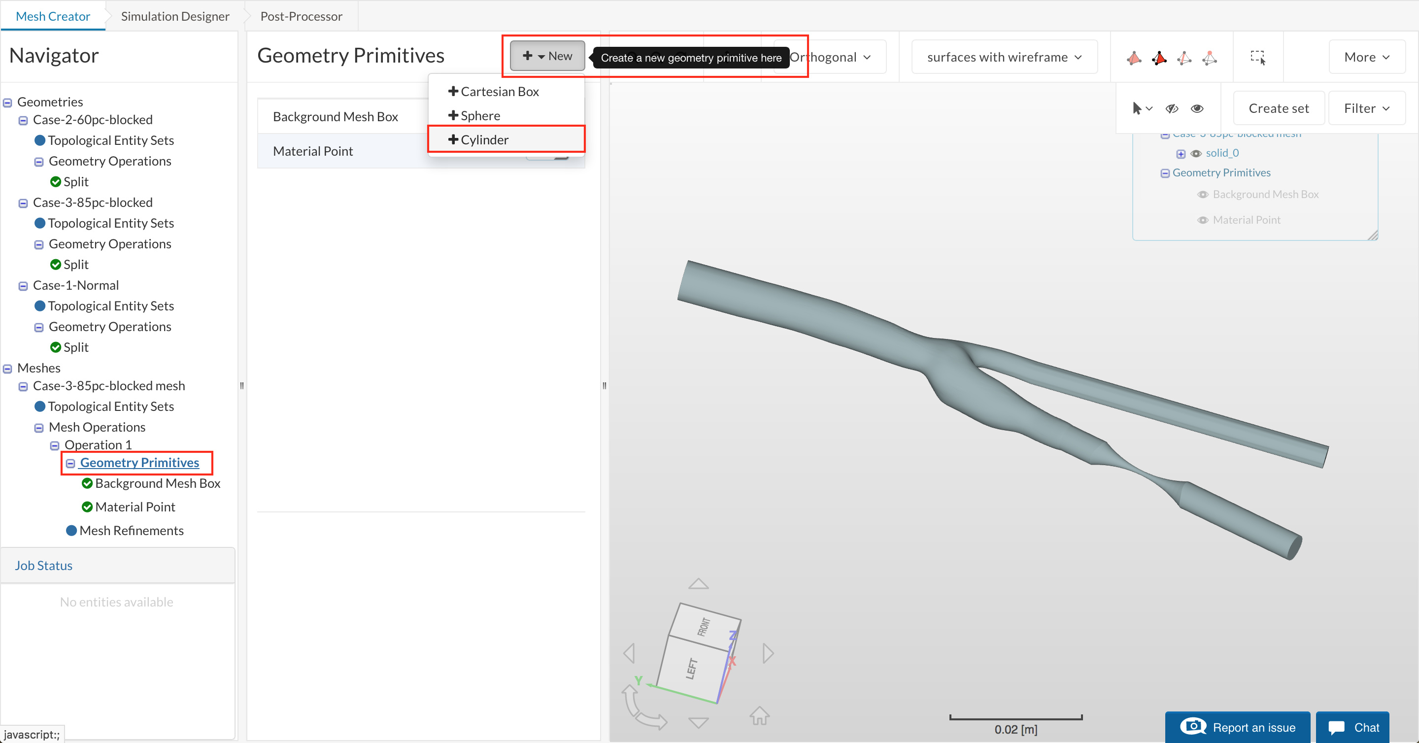
Figure 6: Cylinder primitive creation
Enter the values as shown:
- Reference Point (x): -0.01
- Reference Point (y): -0.043
- Reference Point (z): 0
- Axis (x): 0.0055
- Axis (y): 0.016
- Axis (z): 0
- Radius: 0.003
Click Save to preserve the mesh settings
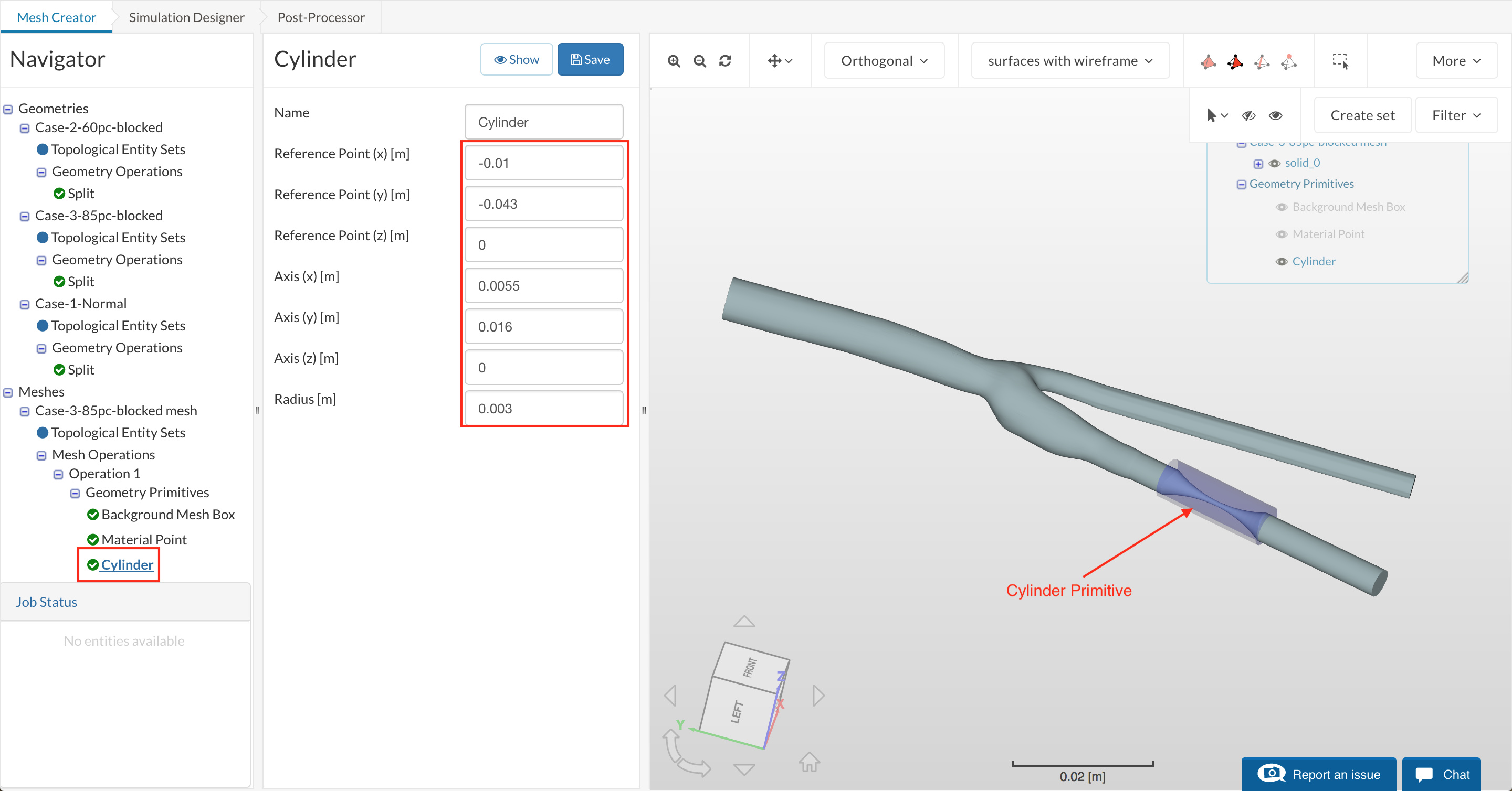
Figure 7: Cylinder primitive settings.
We will now add the necessary mesh refinements for the previously created geometry sets and the geometry primitives.
Click on Mesh Refinements and click +New button to add a refinement.
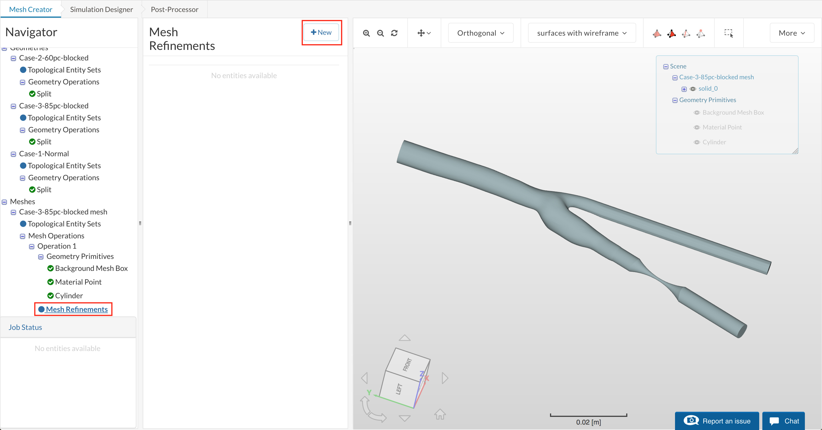
Figure 8: Mesh refinement creation
Ref-surface
This refinement will be used to refine the surfaces for the complete solid geometry. Select the settings as follows:
- Name: Ref-surface
- Type : Surface refinement
- Level Min : 2
- Level Max : 2
- Assigned entity Type: Volume
- Entity: solid_0
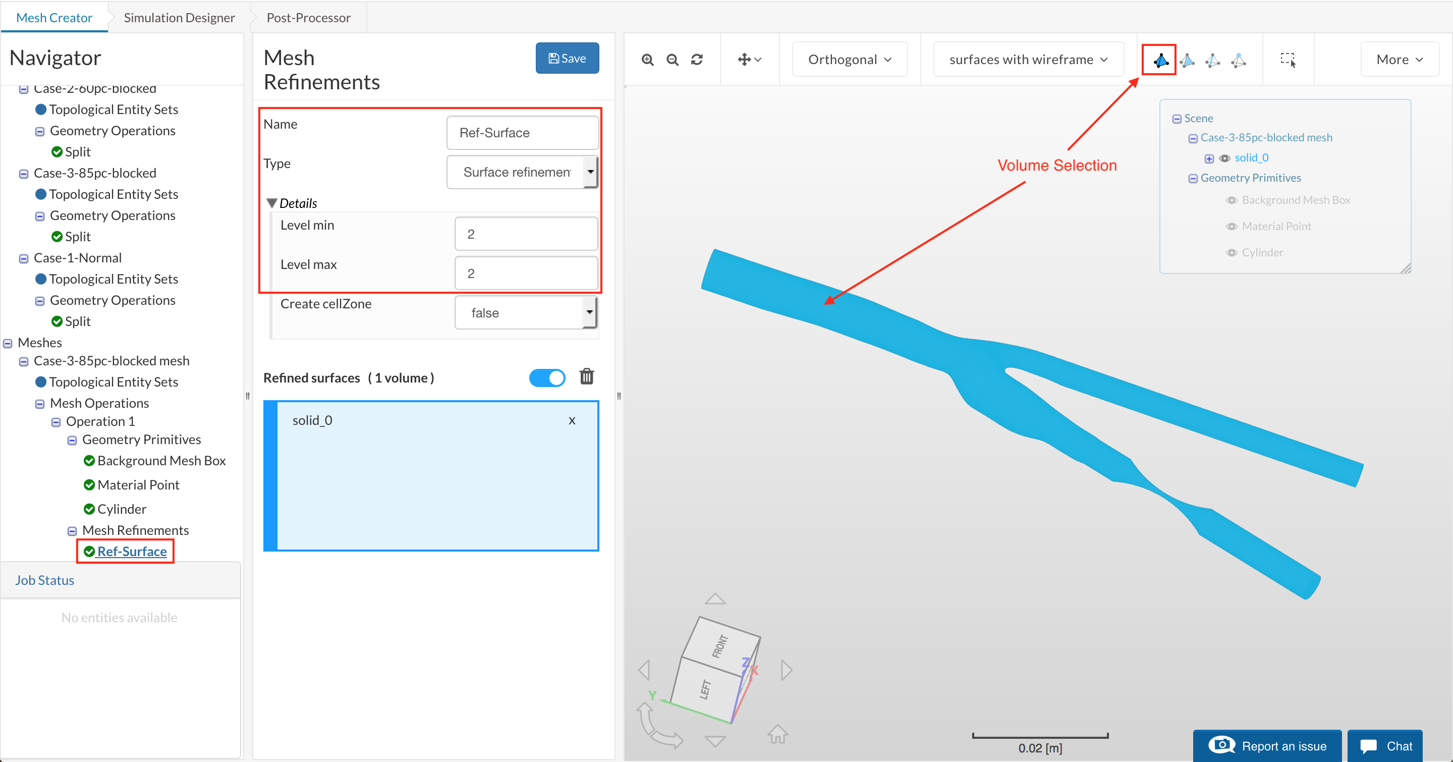
Figure 9: Surface refinement settings and selection.
Click Save to preserve the mesh settings
To create another refinement, hover your mouse over Mesh refinements and right-click to select Add mesh refinement.
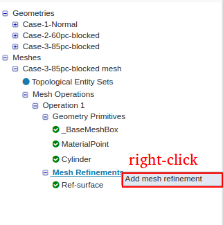
Figure 10: Additional refinement creation.
Ref-layer
The layer refinement is important to capture the behaviour near the wall. This will create layer cells following the surface curvature near the walls.
Add a new Mesh Refinement, and choose:
- Type : Inflate boundary layer
- Change Number of layers: 3
- Keep the rest to default
Under the selection box, select the surfaces:
- shell_0_face_0
- shell_0_face_2
- shell_0_face_3
Click Save
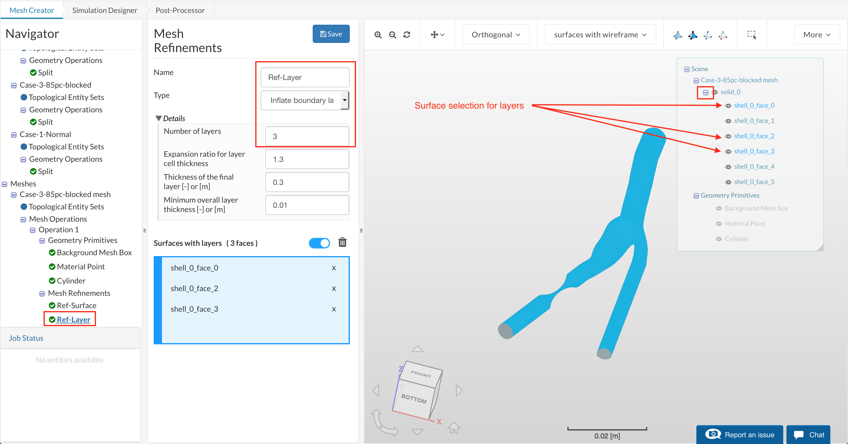
Figure 11: Layer inflation settings and assignements.
Ref-edges
The feature refinement will refine near edges. This is important to capture sharp corners.
Add a New Mesh Refinement, and choose Type as Feature Refinement
Give a Distance of 0.0005 and a Level of 3.
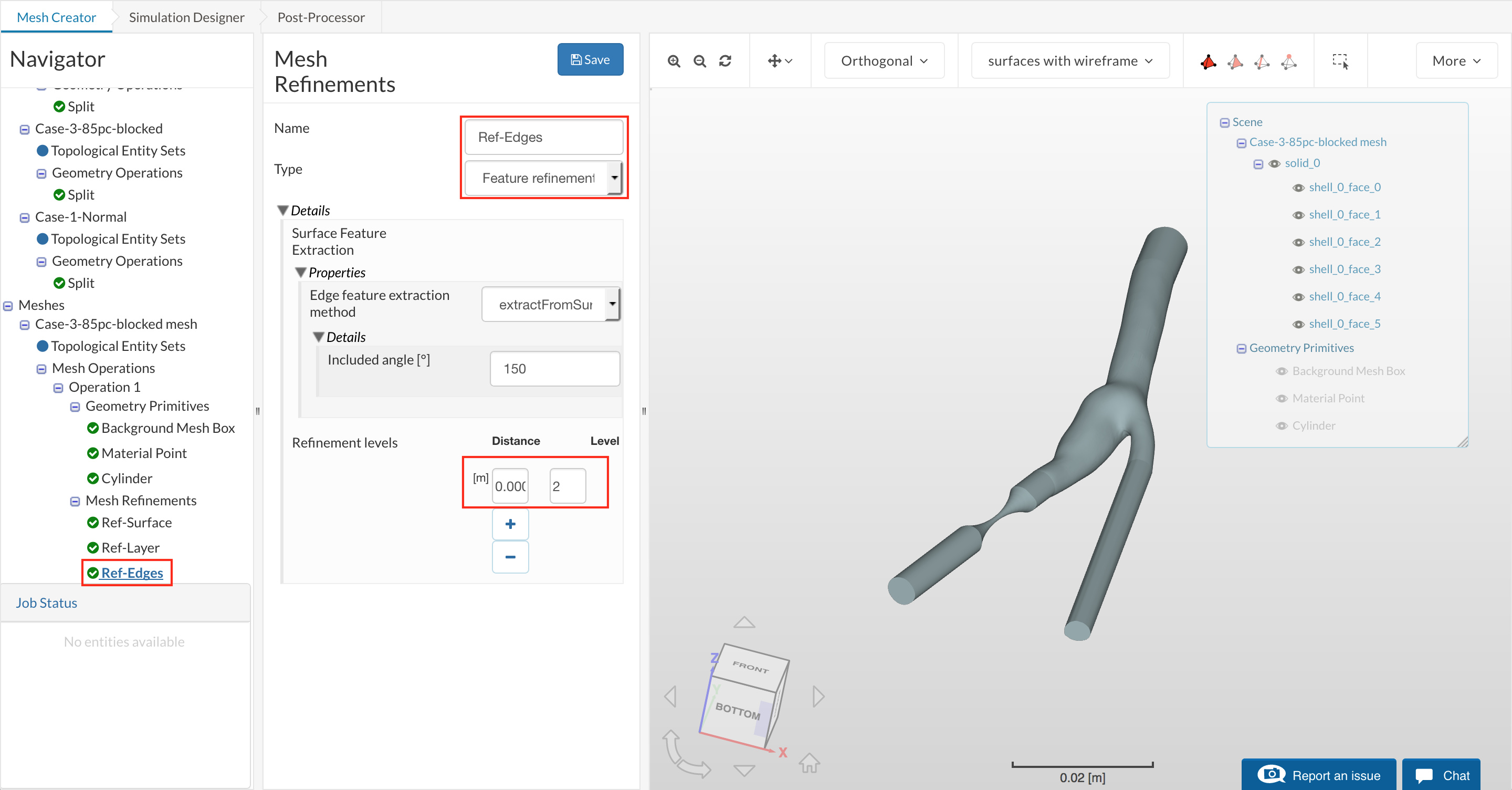
Figure 12: Edge Refinement settings.
Ref-volume-region
These regional refinements will refine the volume mesh. The first is for the entire inner region
Create a new Mesh Refinement enter the settings as follows:
- Name: Reg-volume
- Type : Region refinement
- Mode : Inside
- Distance : 1
- Level : 1
- Under Refined regions box select: solid_0
Then click Save
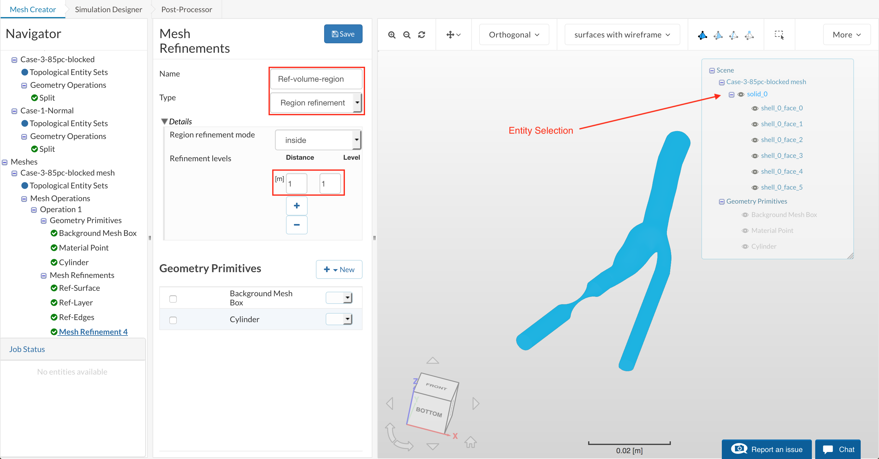
Figure 13: Region refinement settings for solid.
Ref-blocked-region
The next region is for the narrow blocked area. So create another ‘Mesh Refinement’ and enter the settings as follows:
- Name: Reg-blocked
- Type : Region refinement
- Mode : Inside
- Distance : 1
- Level : 3
- Under Assigned Geometry Primitive box select: Cylinder
Then click Save
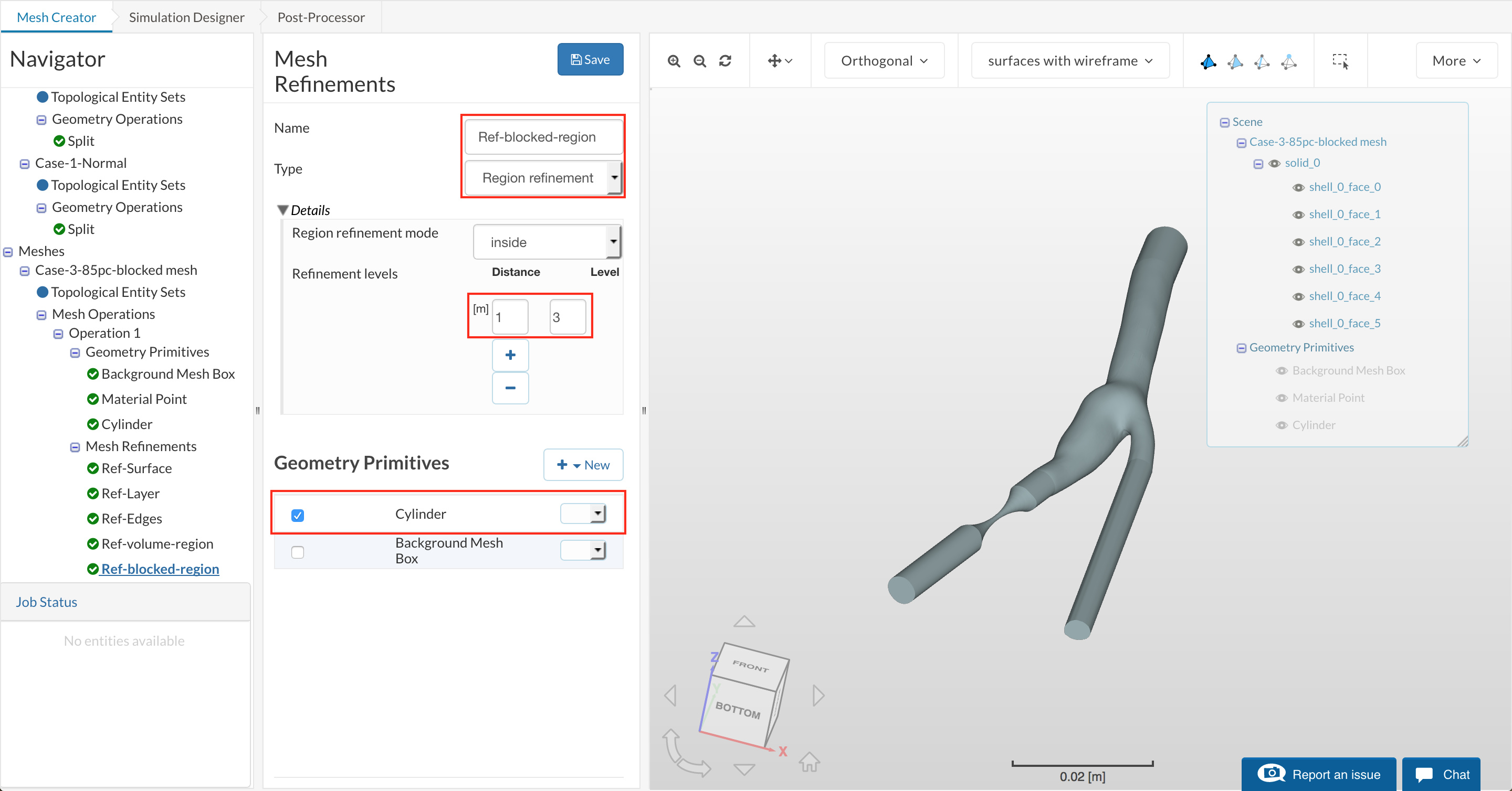
Figure 14: Region refinement settings for blocked region.
Now click back on the main mesh Operation 1, scroll down to the settings panel to Mesh Quality controls and change the 3 parameters as shown and Save:
- Max non-orthogonality angle [°]: 65
- Max concaveness [°]: 70
- Min cell volume [m³]: 1e-18
- Note: This is important to get a good quality mesh.
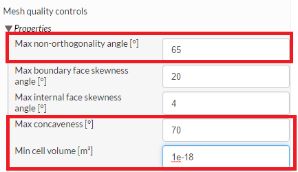
Figure 15: Quality settings to ensure a high-quality mesh is produced.
The mesh settings are all prepared, so click the Start button to begin the mesh generation process. This will take about 5 minutes.
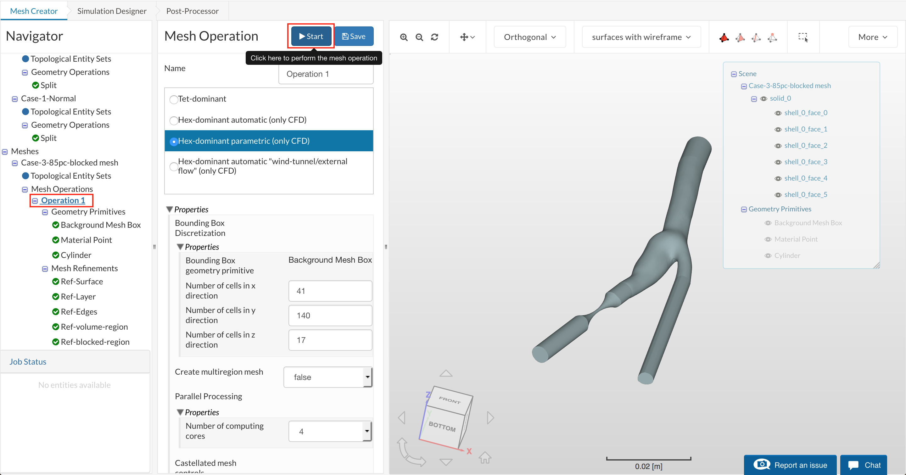
Figure 16: Starting a mesh operation.
Once the process is finished, the mesh is automatically loaded in the viewer.

Figure 17: Finished mesh.
Additional Meshes
Rather than creating meshes for Case 1 and Case 2 from scratch, it is faster to duplicate the mesh you’ve just created and then change the Base Geometry. To duplicate the mesh, just click on the Case-3-85pc-blocked mesh, then right-click and select Duplicate
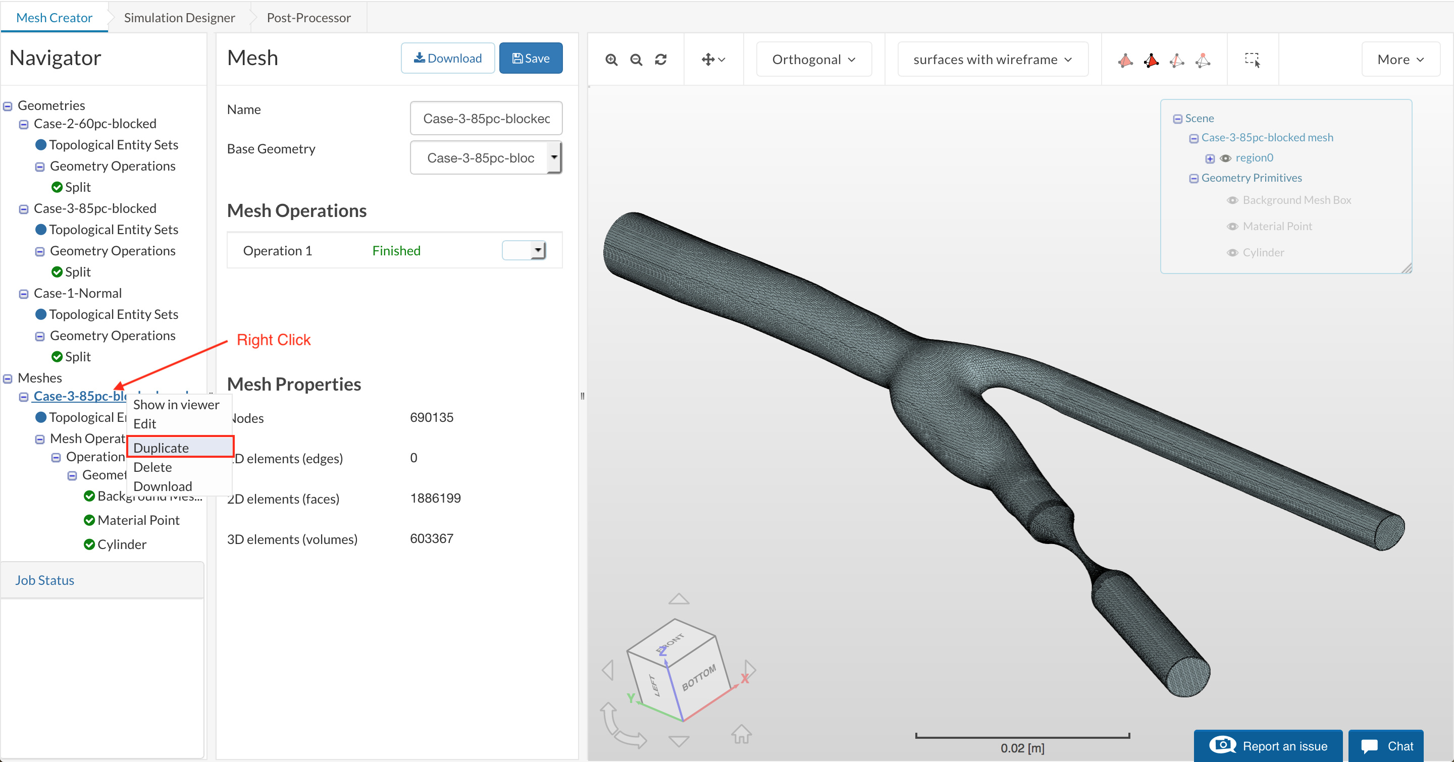
Figure 18: Duplicating the mesh for other cases.
Then click on the duplicated mesh, rename the mesh to Case-2-60pc-blocked mesh, change the Base Geometry to Case-2-60pc-blocked and click Save. (click yes on the confirmation/warning message)
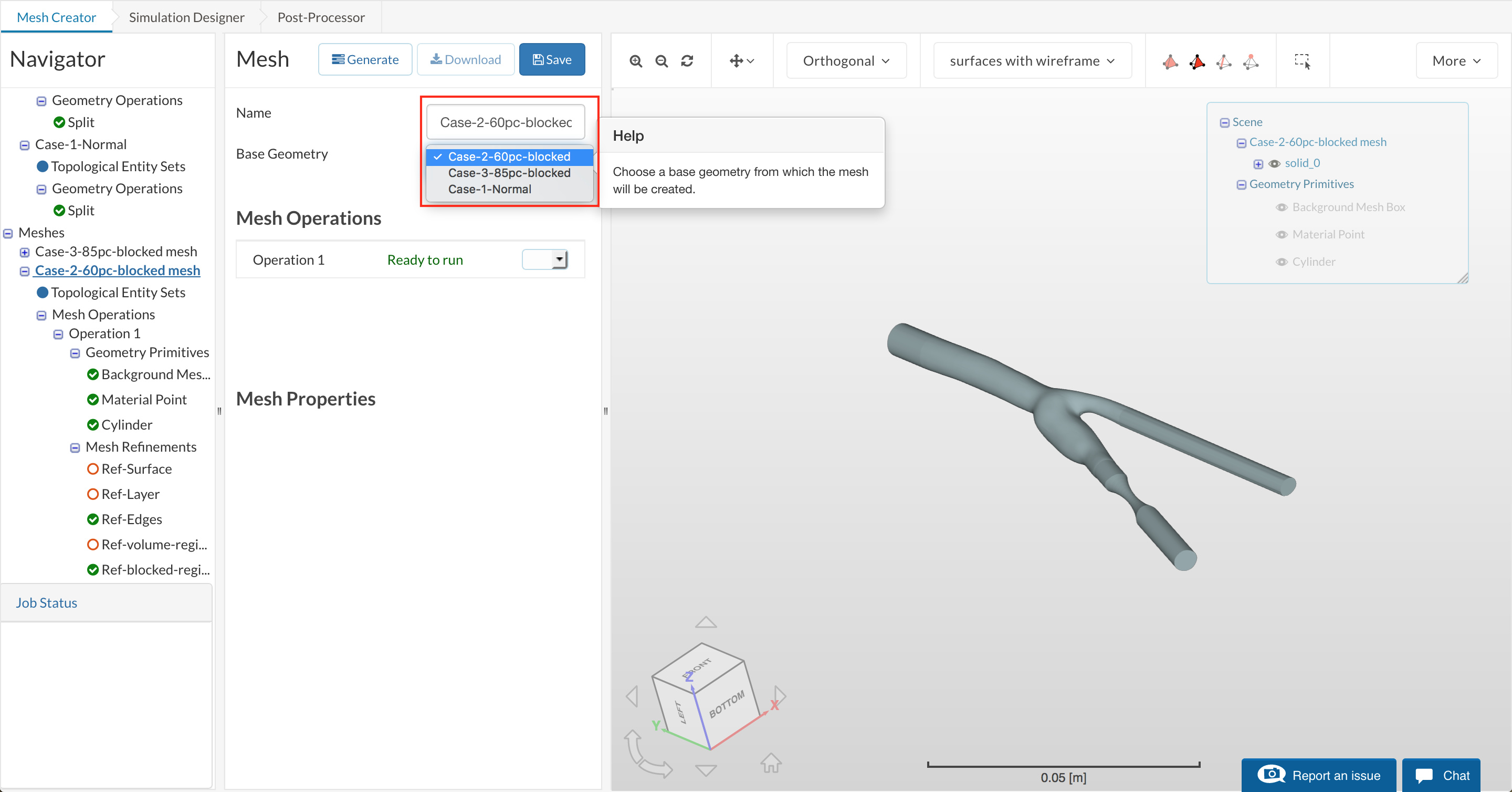
Figure 19: Change name and geometry of the duplicated mesh setup.
Then you will have to Re-assign the corresponding Refinement entities as before.
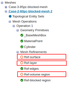
Figure 20: Re-assigning entities to refinements.
Once done go to Operation 1. Click Save and Start to generate the 2nd mesh.
Use the same methodology to create the mesh for Case-1-Normal. Once you have created all 3 meshes, proceed to the next section of the simulation setup.
Simulation Setup
For setting up the simulation switch to the Simulation Designer tab and select +New
Give the simulation a meaningful name: Turb-Steady-blood flow-85pc
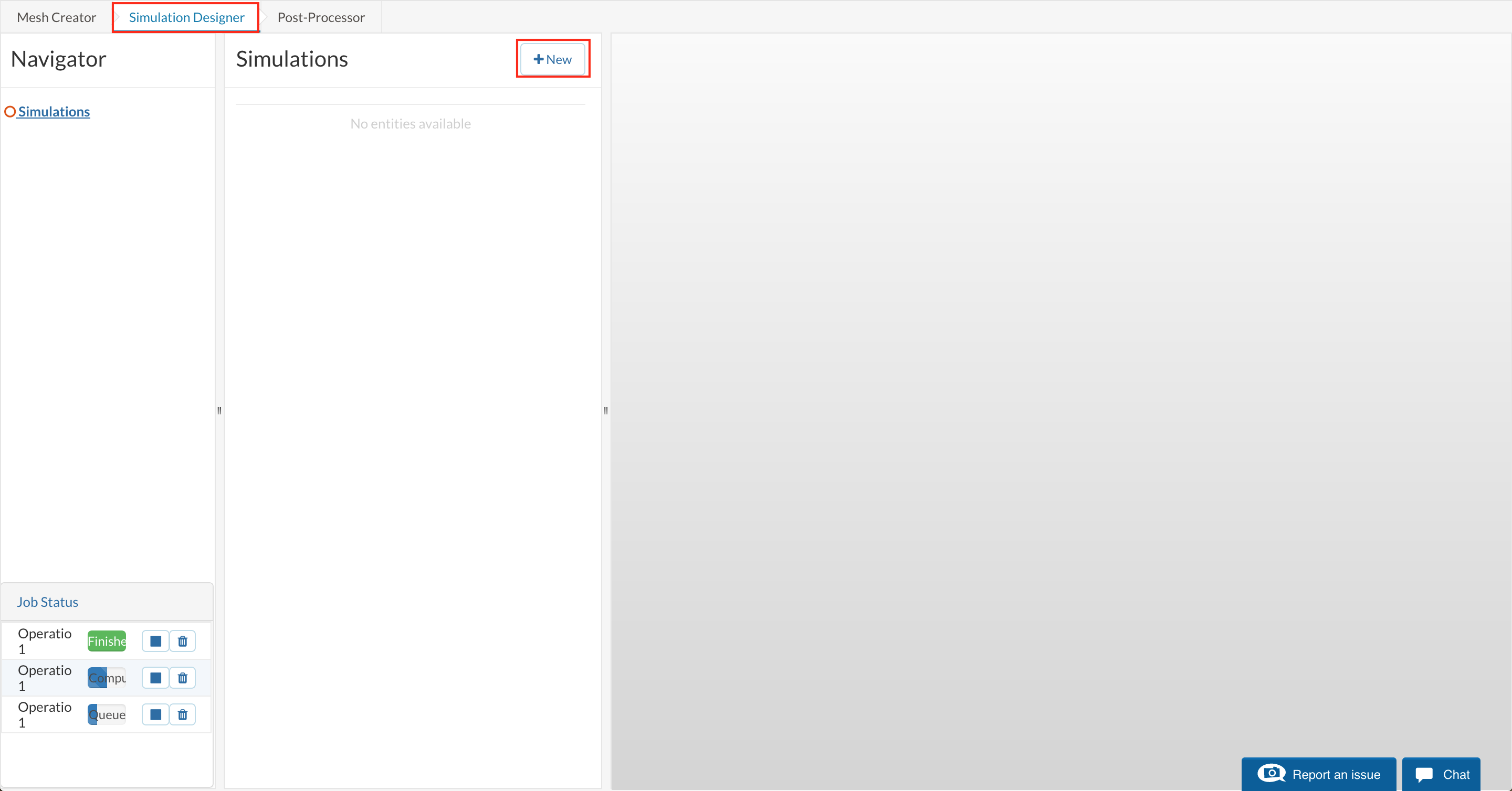
Figure 21: Creating a new Simulation.
Select the analysis type: Fluid dynamics and Incompressible
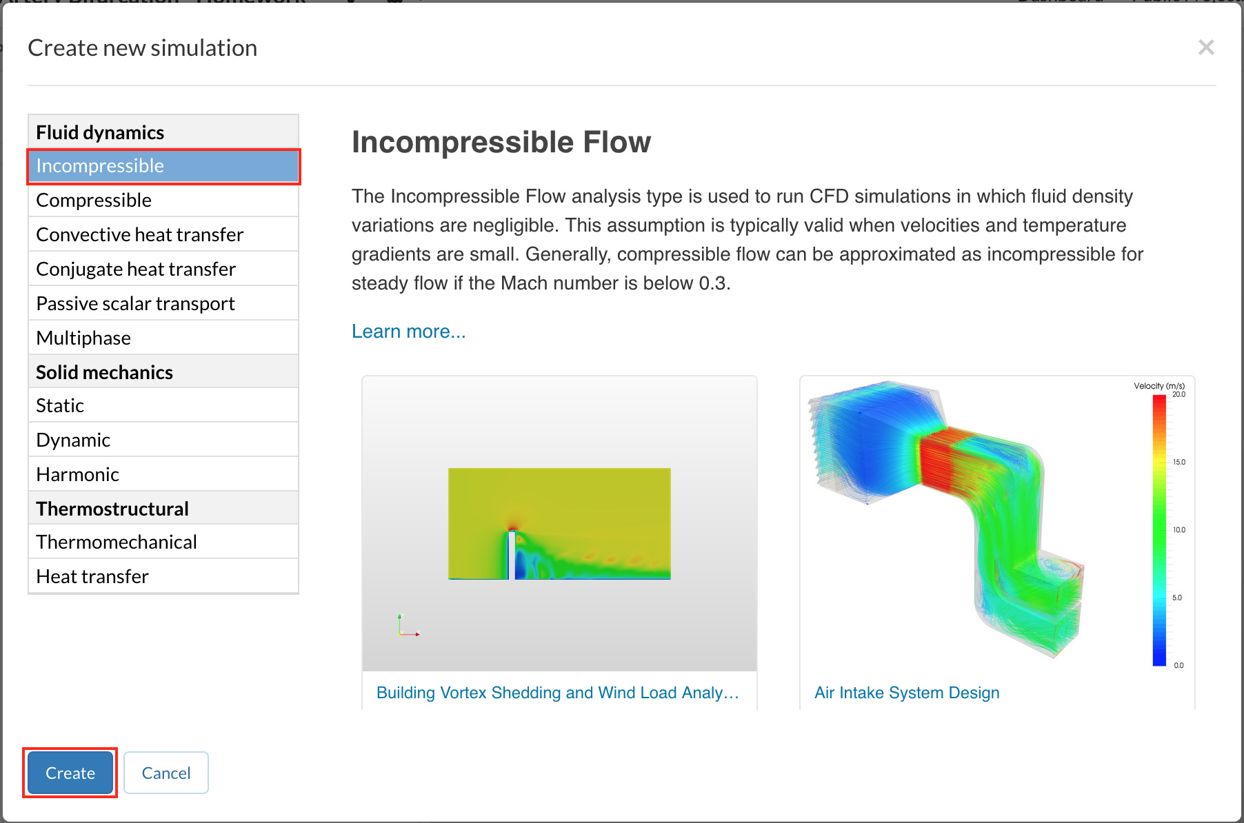
Figure 22: Selecting Incompressible from the fluid dynamics category.
Set the Turbulence model as k-omega-SST and Steady-state. Then click Save.
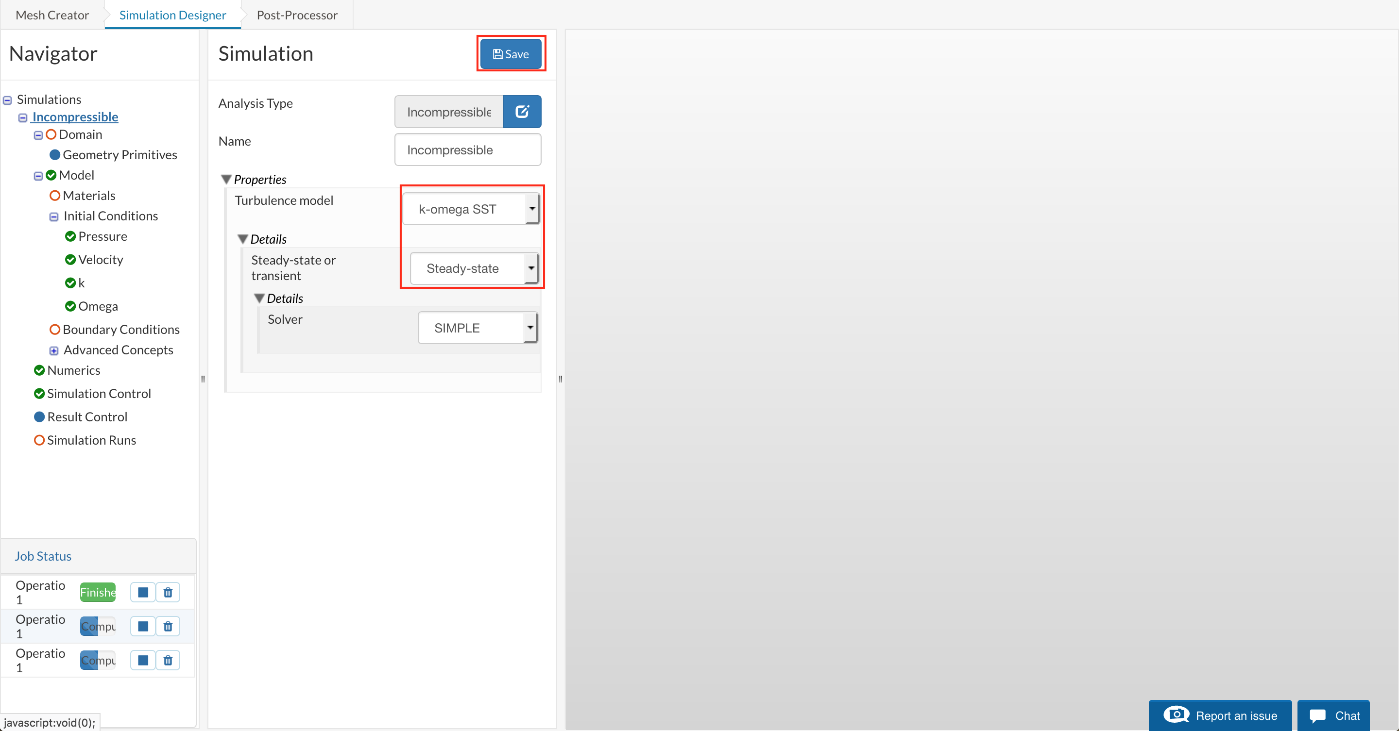
Figure 23: Selecting turbulence model and defining steady state.
After saving, the Navigator now looks as shown below. Here the entries in Red must be completed.

Figure 24: Showing entries in the tree that need to be compleated.
Click Domain from the tree and select Case-3-85-pc-blocked mesh. Click the Save button. The mesh will then automatically load in the viewer.
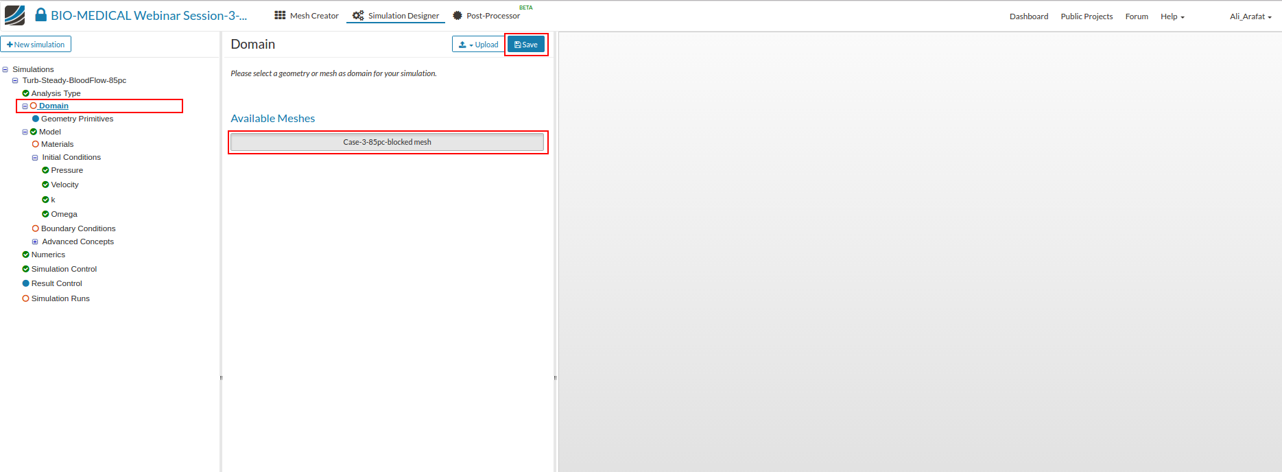
Figure 25: Selecting the mesh under the domain entry.
Now we will create topological entity sets to group the faces together.
Click on the tree entry Topological Entity Sets.
Select the shown face from the viewer (left-click selection), then click the Create set button in the toolbar.
Name the set Common Carotid Artery Inlet.
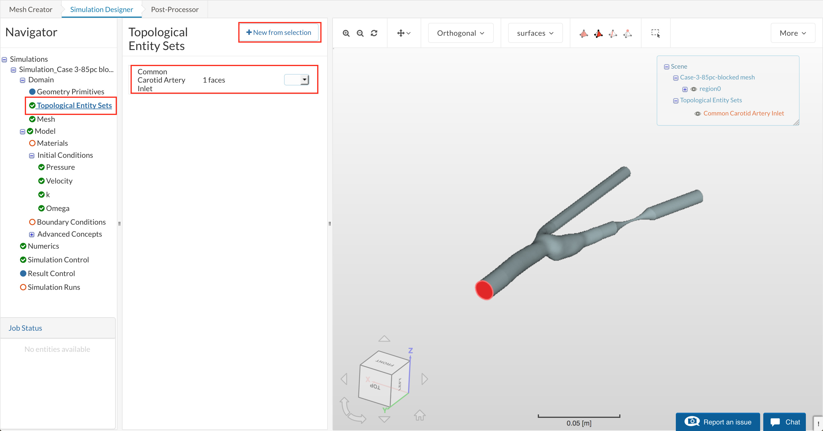
Figure 26: Creating the inlet entity set.
Next, select the 2 shown outlet faces from the viewer, then again click Create set button in the toolbar.
Name the set Carotid Artery Outlets (it has 2 faces)
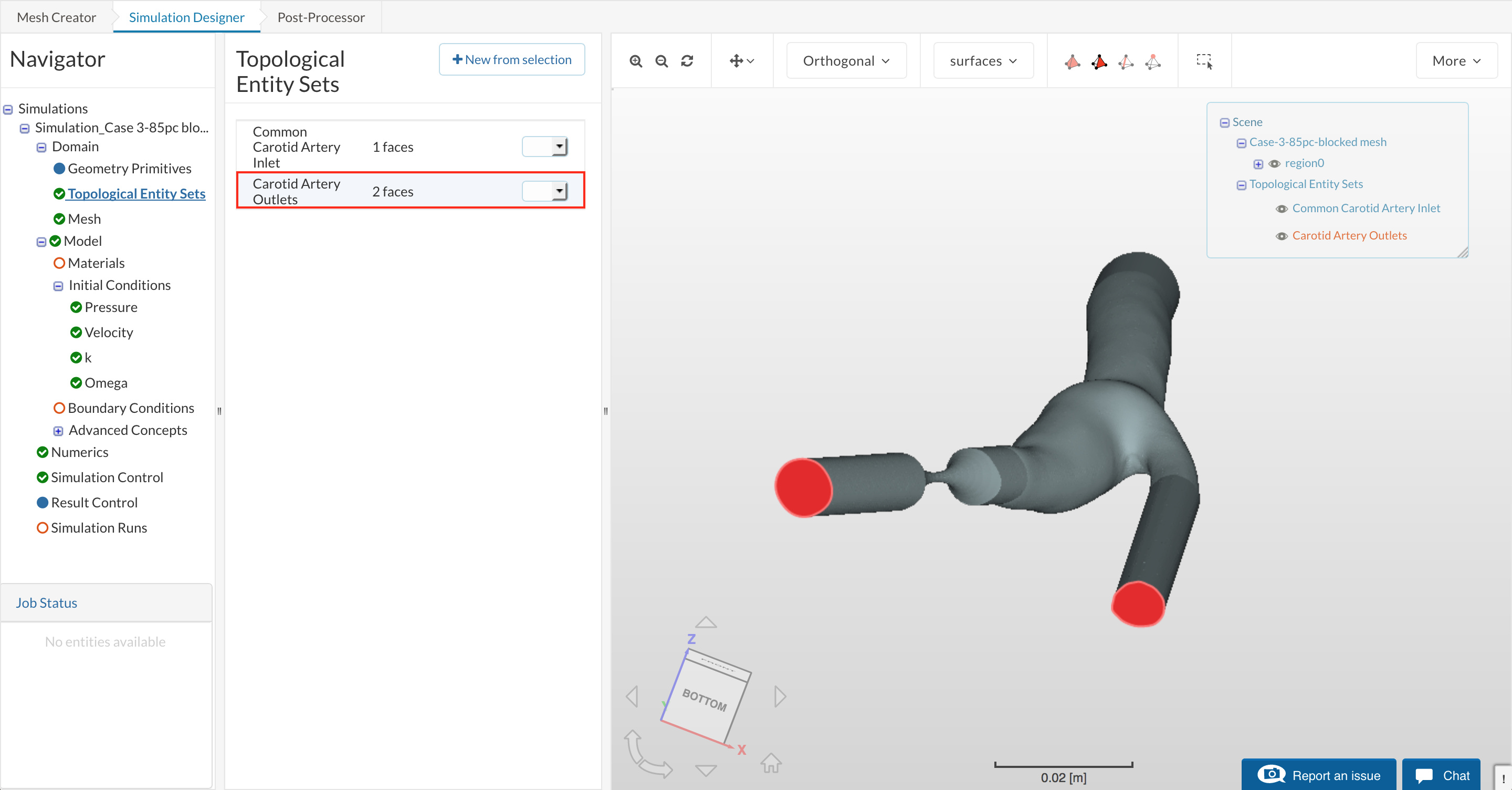
Figure 27: Creating the outlet entity set.
Select both entity sets in the viewer try on the right, right-click in the viewer, and invert the selection. Now create an entity set on the new selection, called *Walls.
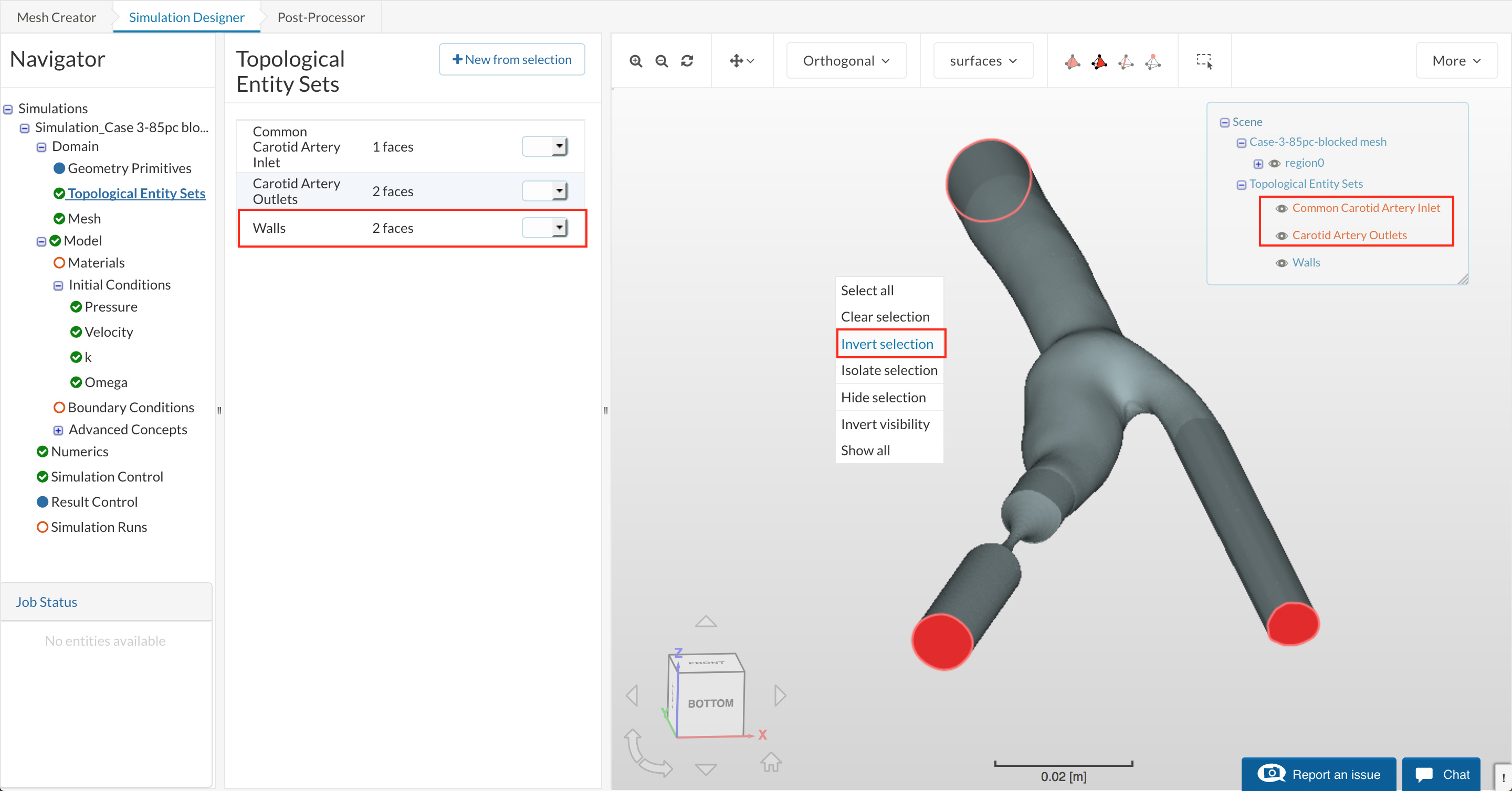
Figure 28: Creating the entity set for the walls.
your selection should show all faces except inlets and outlets selected as depicted below.
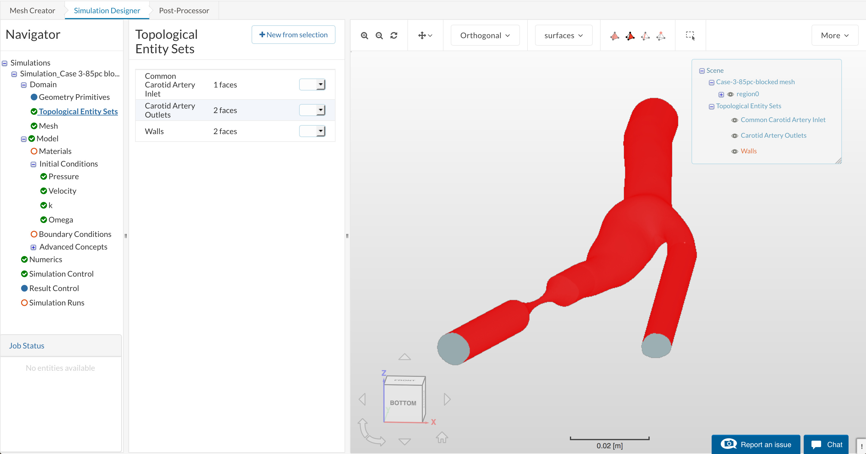
Figure 29: Selection after the inversion.
Once done, you will have three sets with the shown number of faces:
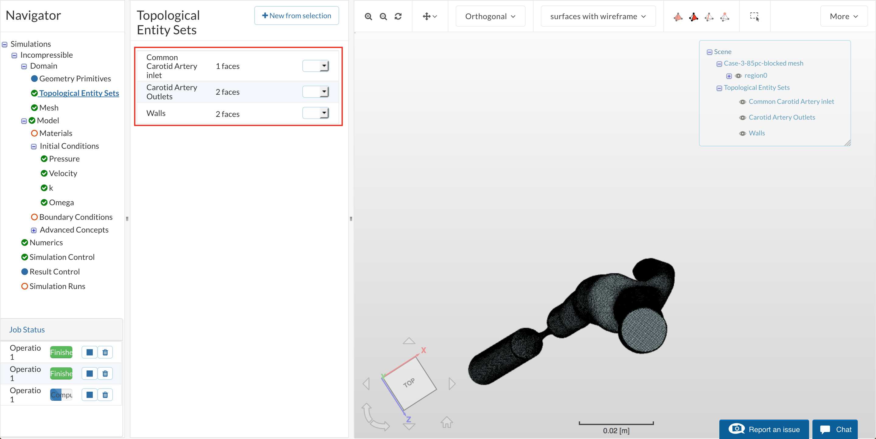
Figure 30: List of entity sets with expected number of faces.
We now add a Fluid material (Blood). Select the Material item in the Navigator and click New

Figure 31: Creating a new material (Blood).
Specify the given properties to define the non-newtonian model for blood (for details see Documentation):
- Viscosity model: Bird-Carreau
- Viscosity at zero shear nu0 [m²/s]: 0.00005283
- Viscosity at very high shear nuInf [m²/s]: 0.0000032547
- k [s]: 3.313
- n [-]: 0.3568
- a [-]: 2
- Density [kg/m³] = 1060
Now to assign this fluid to the mesh domain, select the available domain called region0 and click save.
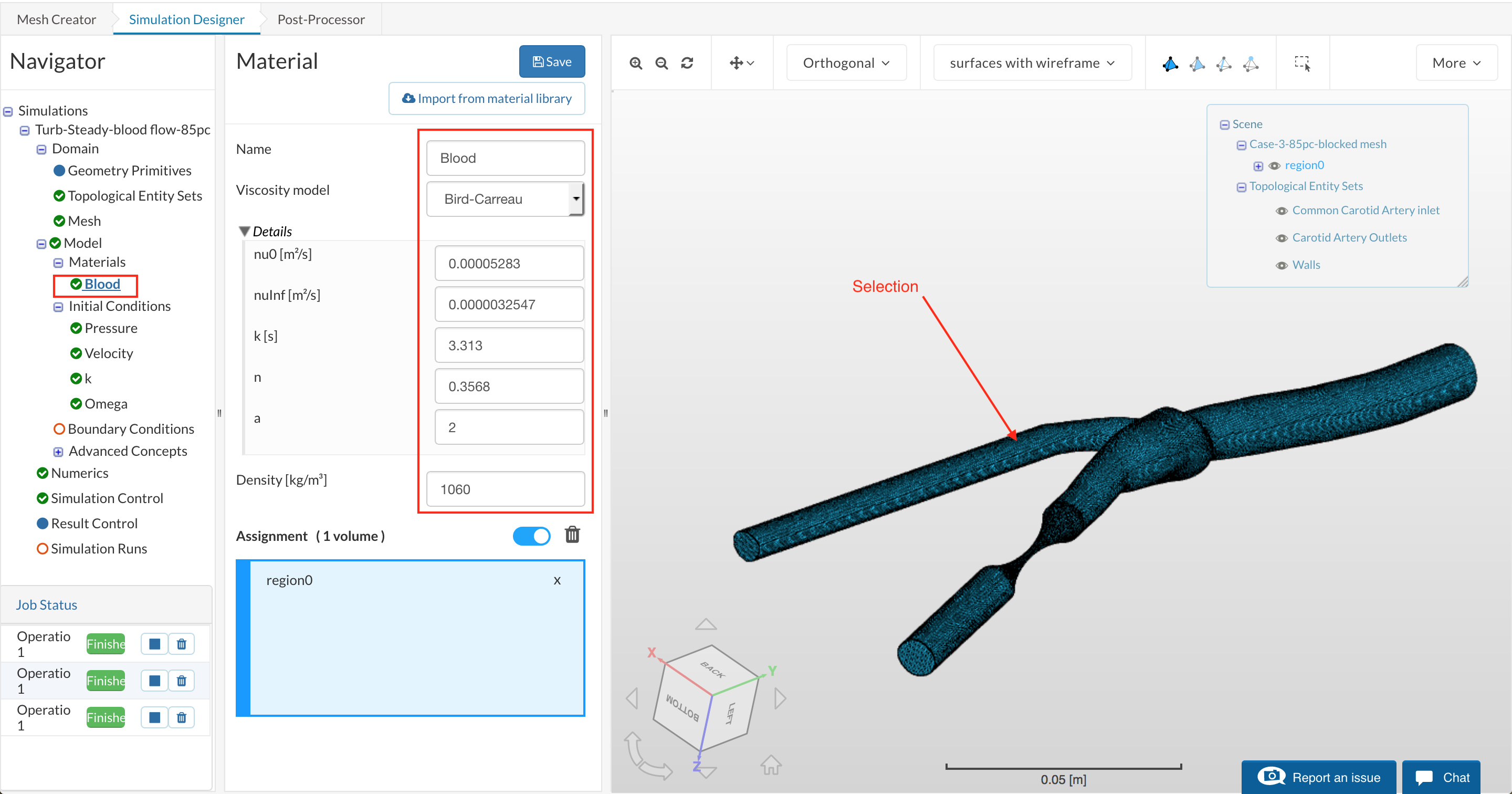
Figure 32: Specifying the material Blood and assigning it to region0.
The boundary conditions define the flow variables at the boundary surfaces.
Click on Boundary condition and select +New.
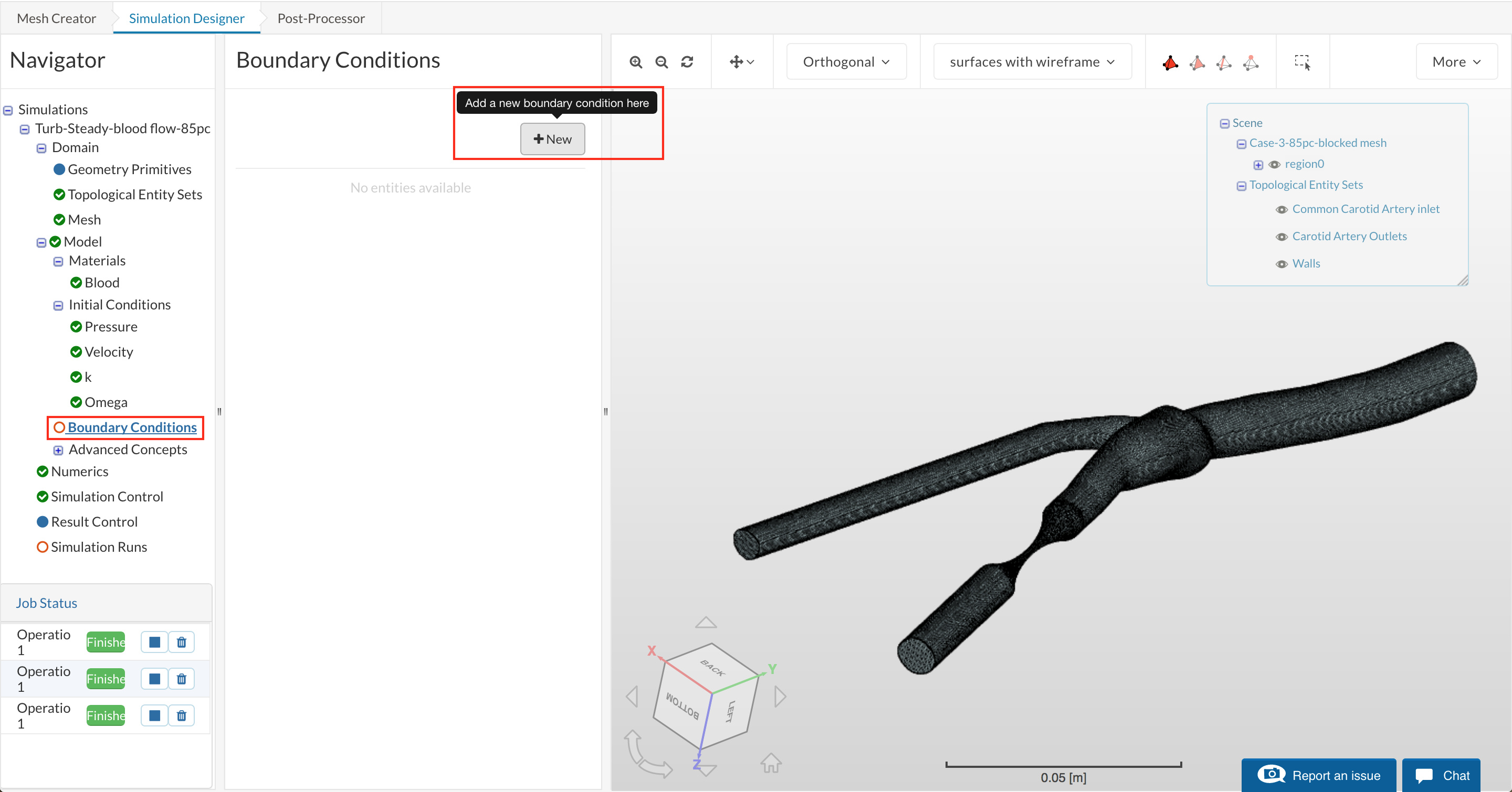
Figure 33: Creating a new boundary condition.
Inlet
Select the Type as Pressure Inlet, and Type as Total Pressure
Gauge Total Pressure [Pa]: 1184
Pressure difference was taken using a known flow rate through a healthy artery and applied to the inlet to ensure pressure driven flow. Pressure can be applied to the inlet and zero pressure at the outlet since this is an incompressible flow simulation.
From the selection box, select the previously created Common Carotid Artery Inlet and click Save
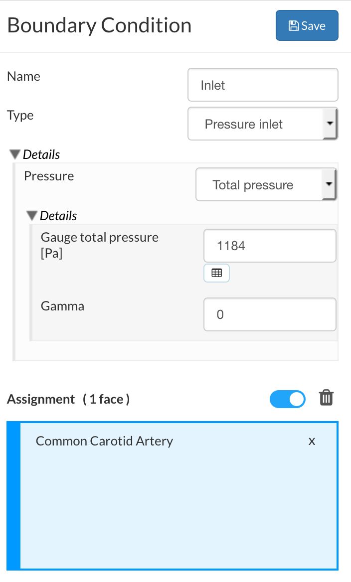
Figure 34: Specifying the settings for the Pressure Inlet.
Outlet
Add another boundary condition, select the Type as Pressure Outlet and keep the other parameters as default. (here the zero value is only a reference)
From the selection box, select the previously created ‘Outlet set’ and click Save
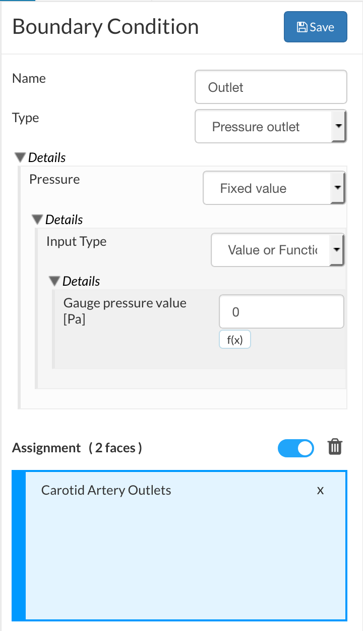
Figure 35: Specifying the settings for the pressure outlet.
Artery walls
Lastly, add another boundary condition for the Artery walls.
Select the Type as Wall, velocity as No-slip and change the wall treatment to zeroGradient
From the selection box, select the previously created Artery walls topological entity set and click Save
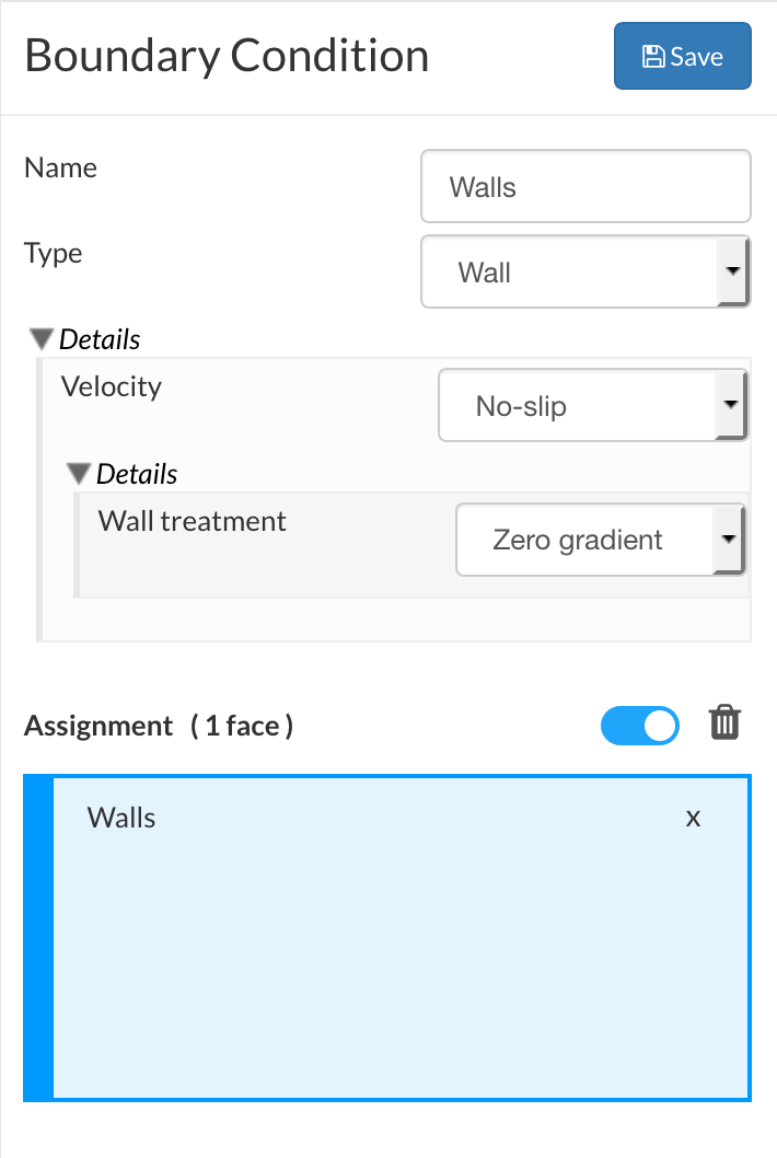
Figure 36: Specifying the settings for the Artery Walls.
Under the Numerics item in the Navigator, make the following changes to improve the solution accuracy.
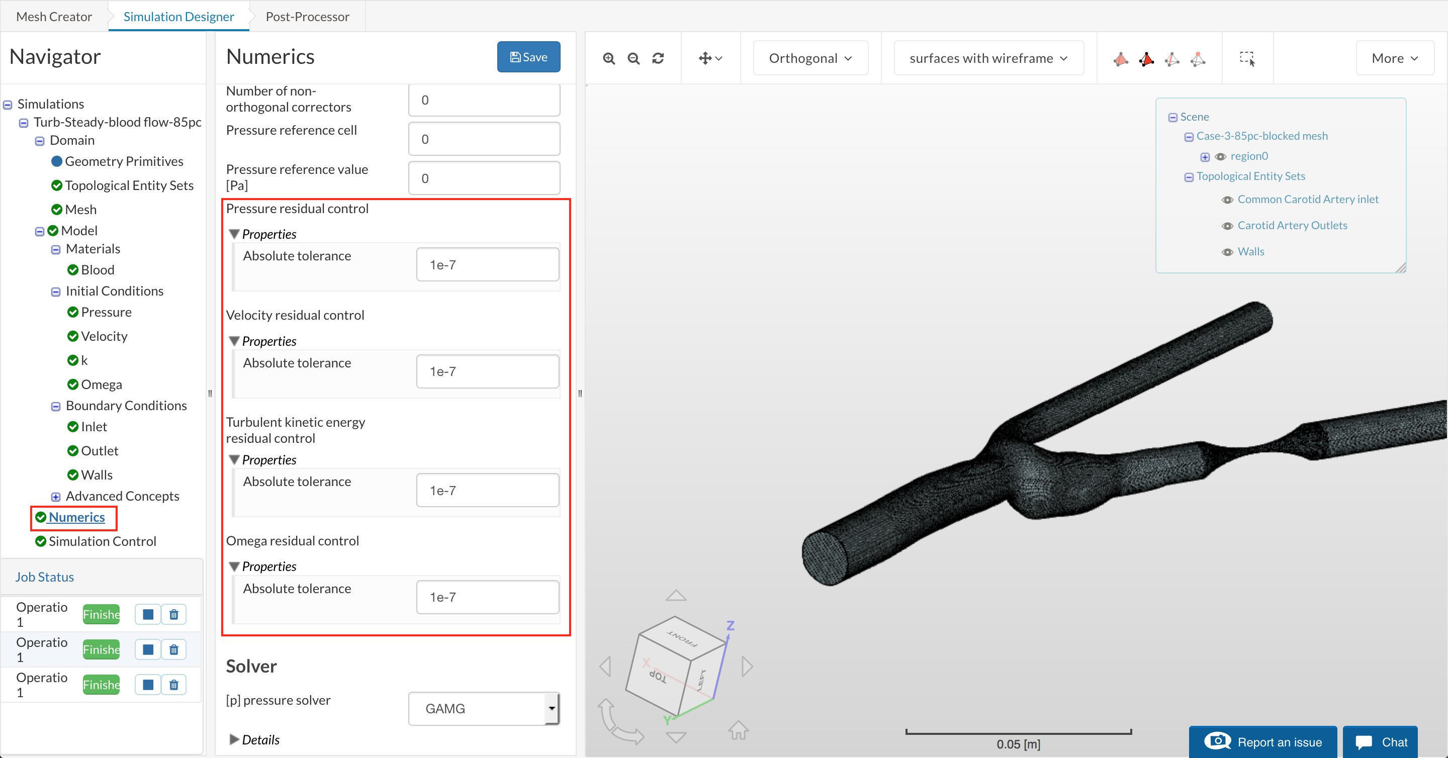
Figure 37: reducing the termination criteria for all residuals.
Under Simulation Control set the parameters as follows:
- Start time value [s]: 0
- End time value [s]: 4000 (these are basically iterations for steady state analysis)
- Time step length [s]: 1
- Write control : Timestep with Write interval (simulation time steps)=2000 (to save only the final solution)
- Number of computing cores: 8
- Maximum runtime [s]: 9000
- Initialize with potential flow: false
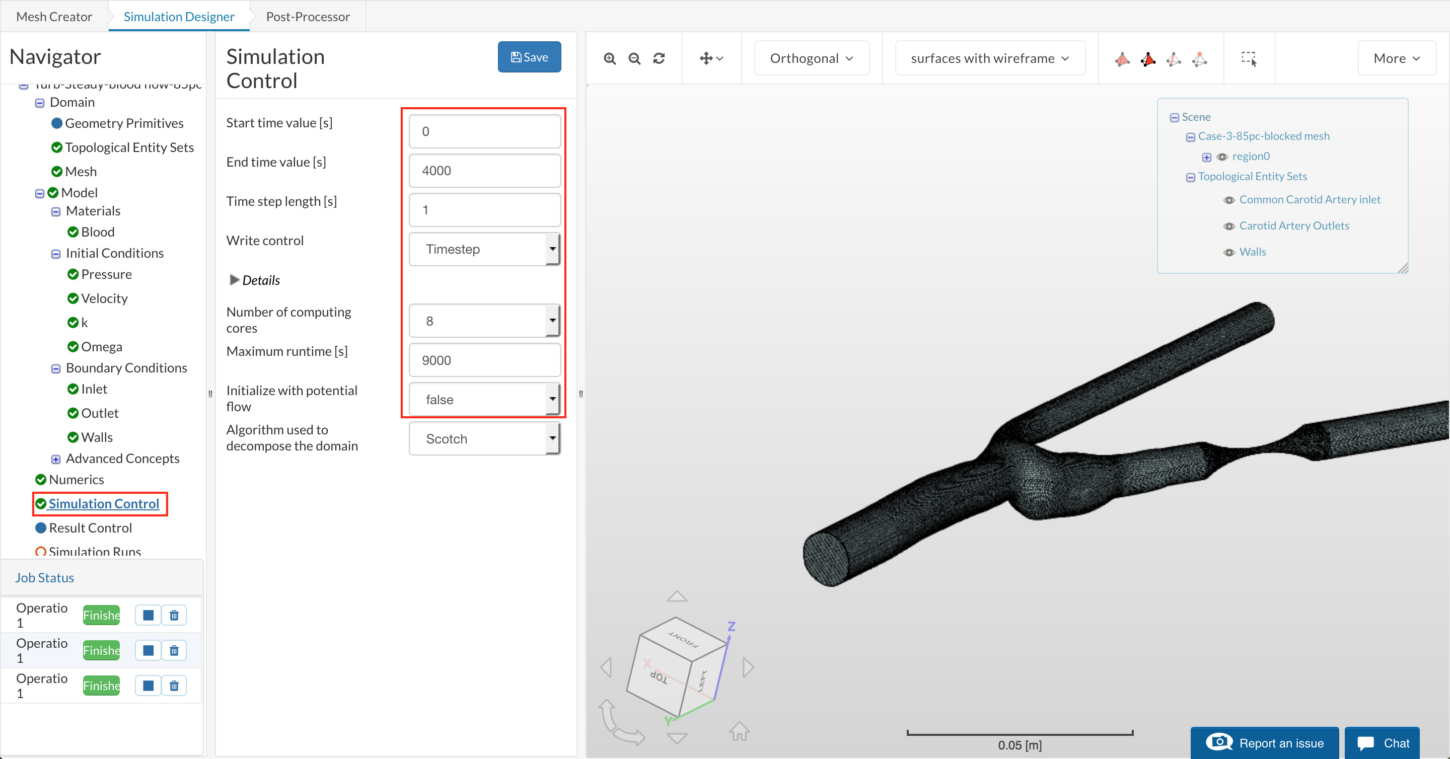
Figure 38: Adjusting the Simulation Control Settings to ensure convergence is reached.
Result Control
Click on Result control and add a Surface Data result control Item. Change the name to Integrals and type to Area Integral. Set it to update every 10 iterations and select the Common Carotid Artery Inlet as the surface. This will measure the volume flow rate through the artery.
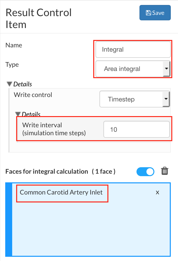
Figure 39: Defining the surface Integral result control item.
Simulation Runs
Click on Simulation runs and create a New run.
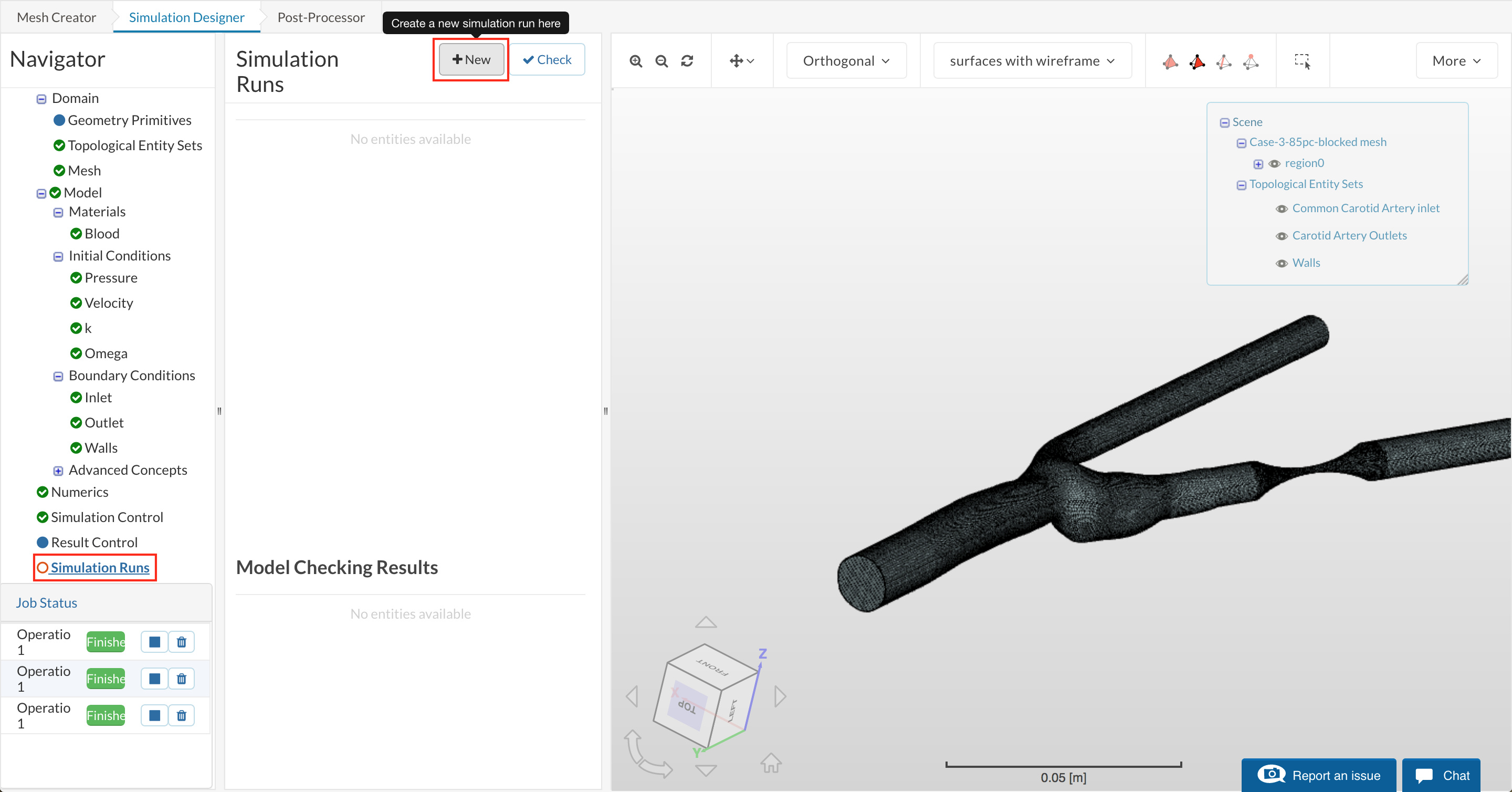
Figure 40: Creating a new run on the selected simulation.
The run should automatically start.
The simulation will take around 40 minutes to Finish. Once finished, the results can then be viewed.
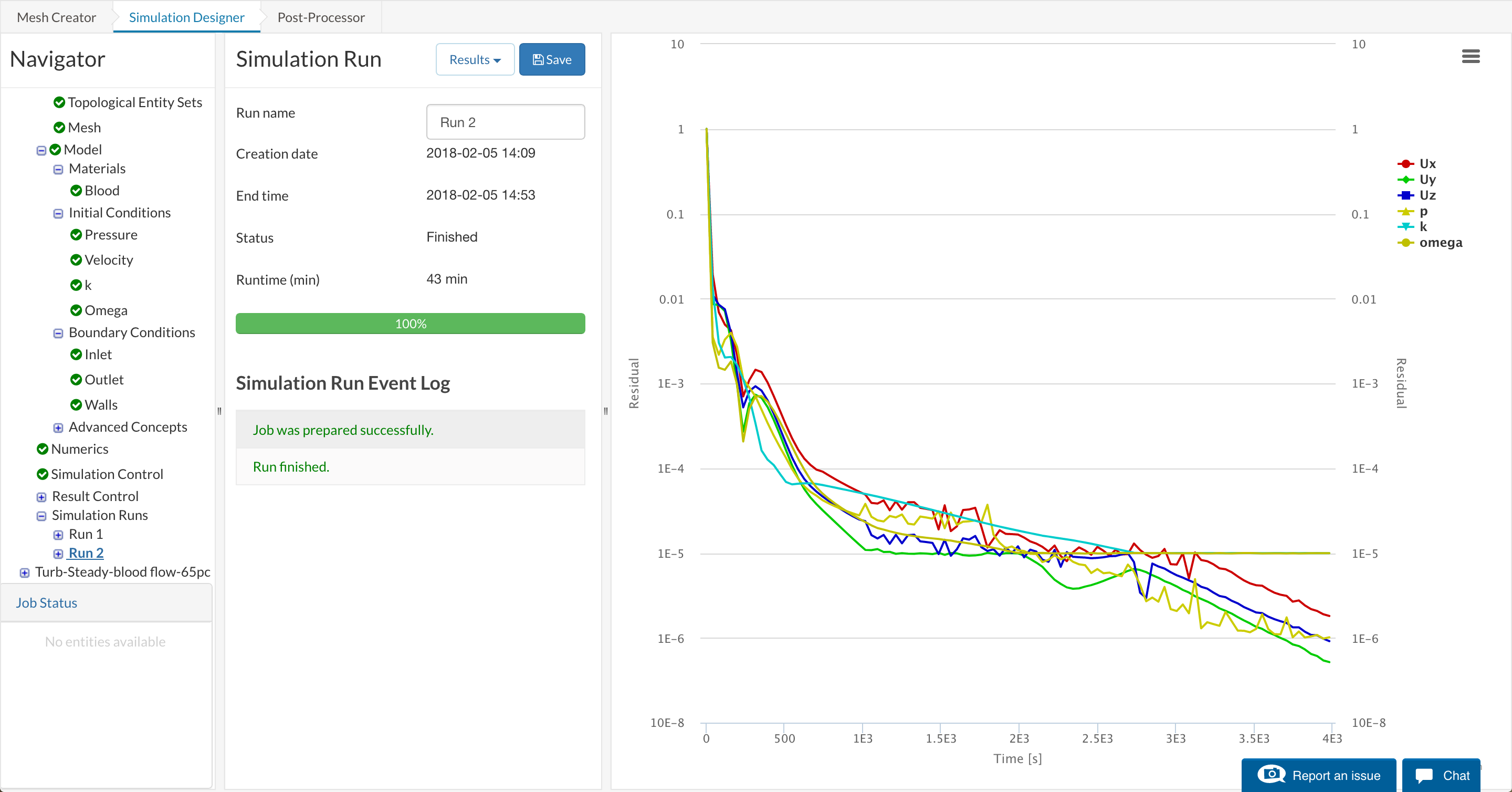
Figure 41: Convergence plot of a finished run.
Additional Simulations
To set up the simulations for the other 2 configurations, you can duplicate the first simulation setup by right-clicking on the Turb-Steady-blood flow-85pc and select Duplicate. Then continue by selecting the appropriate mesh (Case-2-60pc-blocked mesh or Case-1-Normal mesh) under the Domain item in the Navigator and following the previous steps.
Post-Processing
To view the results, switch to the Post processing tab.
Click on Solution fields under Run1 in the navigation tree to load the results. This will take a minute or more depending on the internet speed. Once loaded it will be as shown in the figure below.
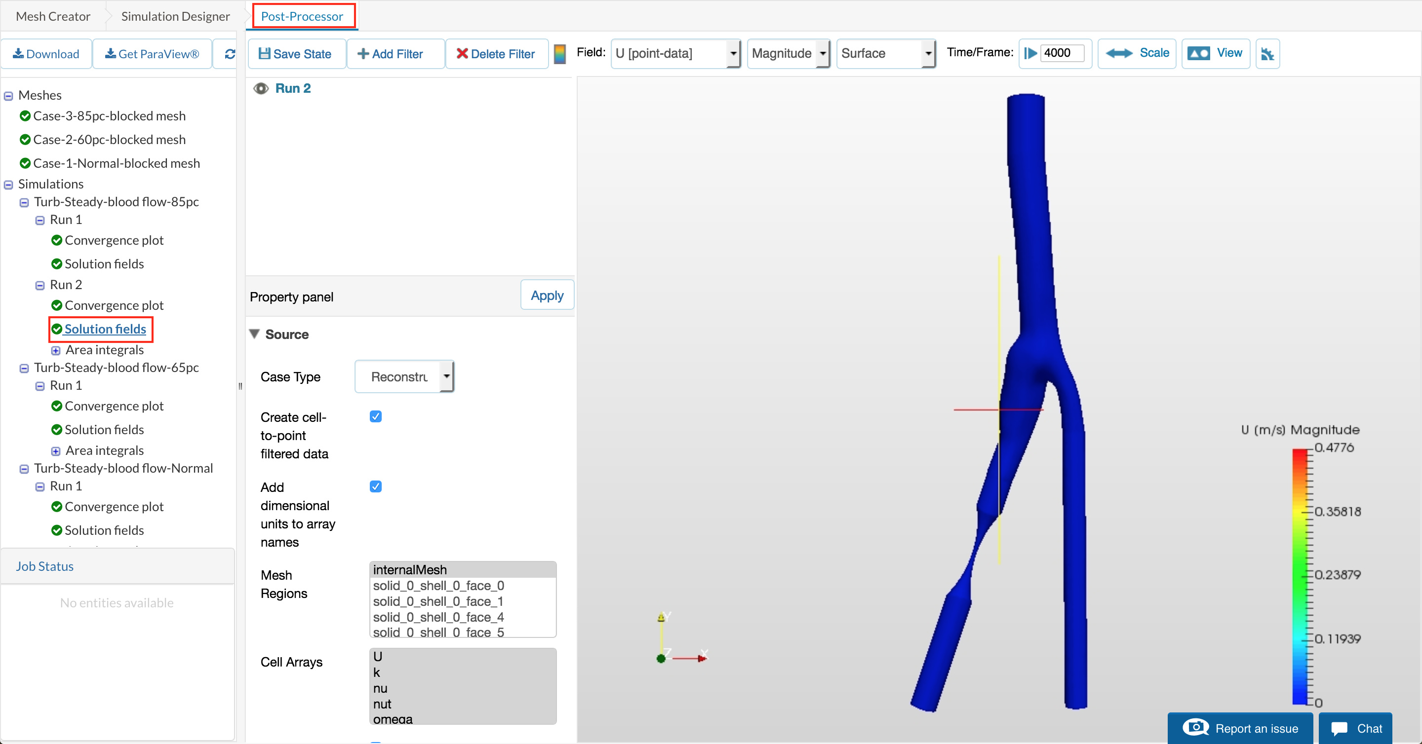
Figure 42: Bring a solution into the Post-processor viewer.
To visualize the internal region we will create 3 Slice filters.The parameters for each are given in the table below:
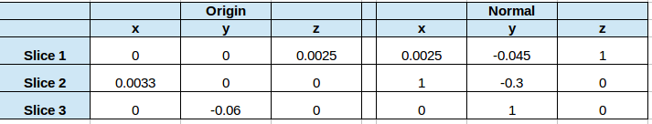
Table 1: Table of slice filter settings for slices 1, 2 and 3.
Slice Filter
To create a Slice filter, click on Run 1 and then the Add filter button. Select the Slice option.
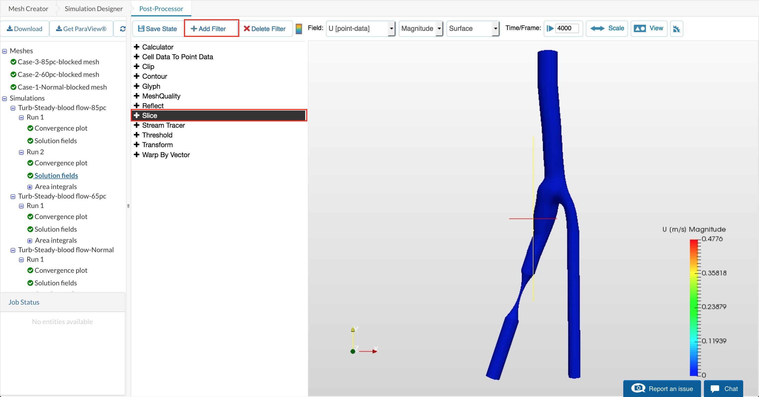
Figure 43: Add a slice filter from the drop down list.
Wait for the filter to apply. Then enter the parameters for Origin and Normal as given in the table.
Uncheck the option Show Plane and click Apply
From the fields drop down (top-left corner) select U [point-data] to view velocity magnitude.
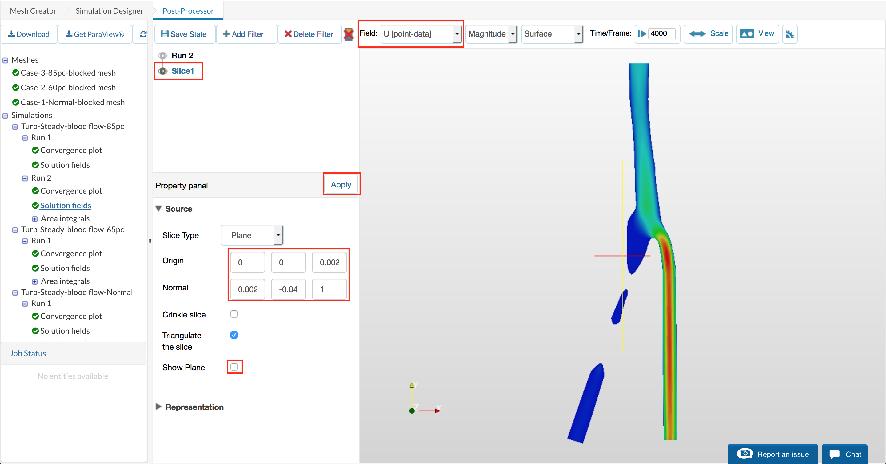
Figure 44: Slice filter 1 showing velocity magnitude.
Follow the same procedure to create the Slice 2 and Slice 3. After creating the 3 Slices, the results will look as shown below (Note: be sure to create each slice from Run 1):
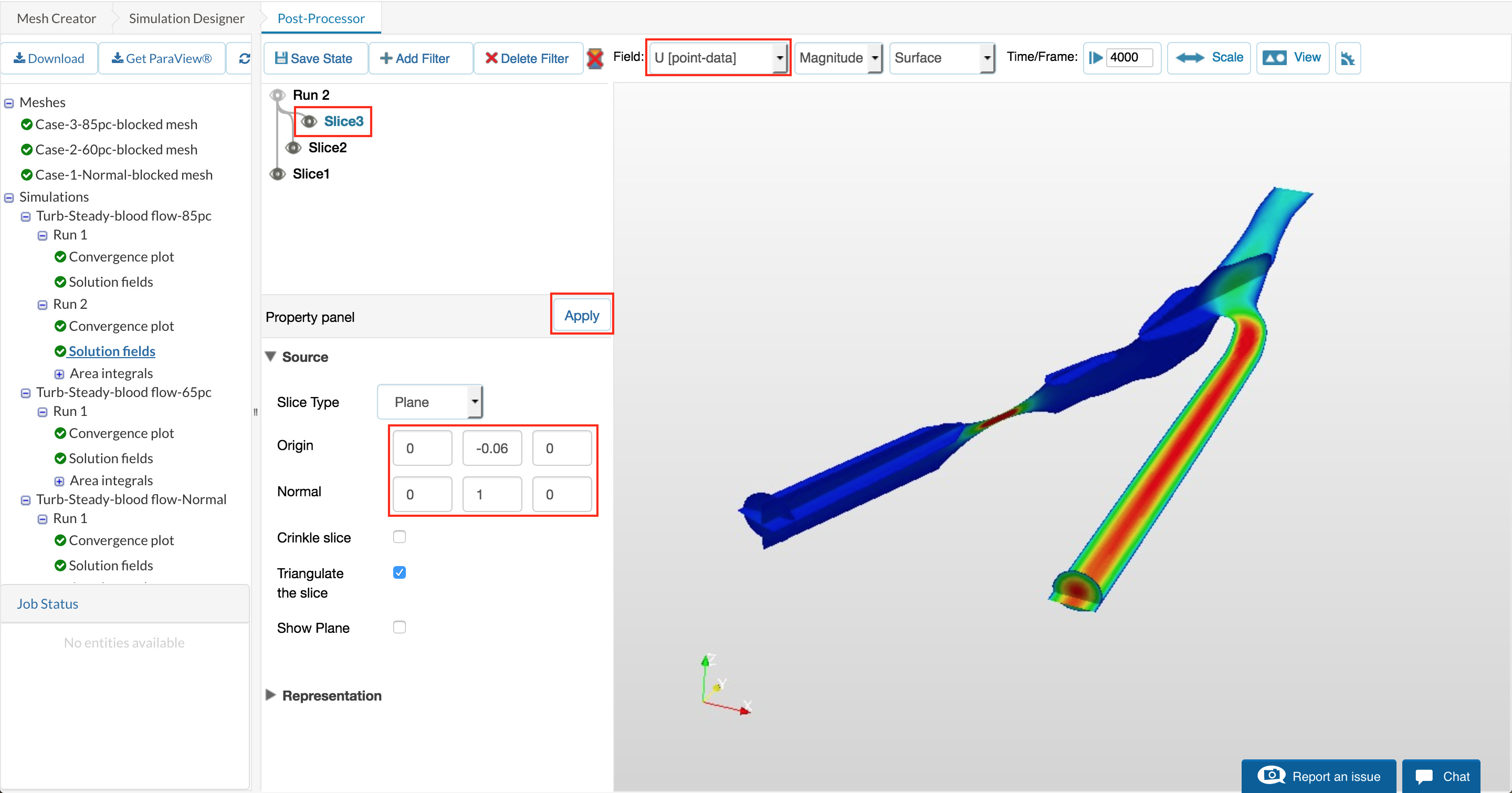
Figure 45: Showing slices 1, 2 and 3 coloured by velocity magnitude.
To view the body walls, click again on Run 1 as shown and click the eye icon to turn it on.
From the fields drop down (top-left corner) select solid color
Then in the properties, under Representation, change Opacity to 0.3 and click Apply
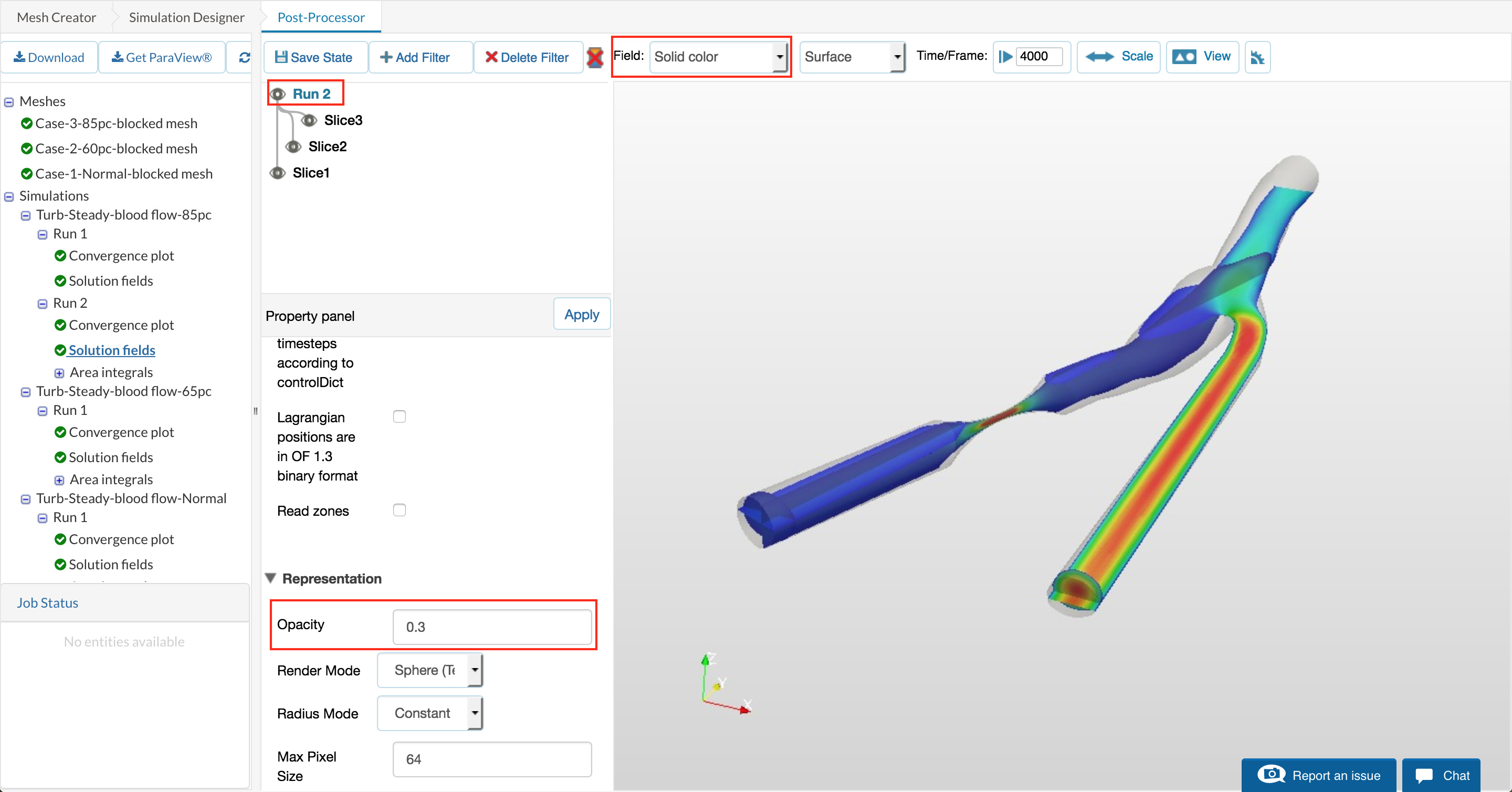
Figure 46: displaying the geomitry as a transparend solid object to add context to filters.
Streamlines Filter
Click again on Run 1 (highlighted in blue) and Add filter to select Stream Tracer
Wait for the filter to apply. Then enter the parameters as below:
- Center: 0.0025, 0.001 , 0.0025
- Radius: 0.003
…and click Apply
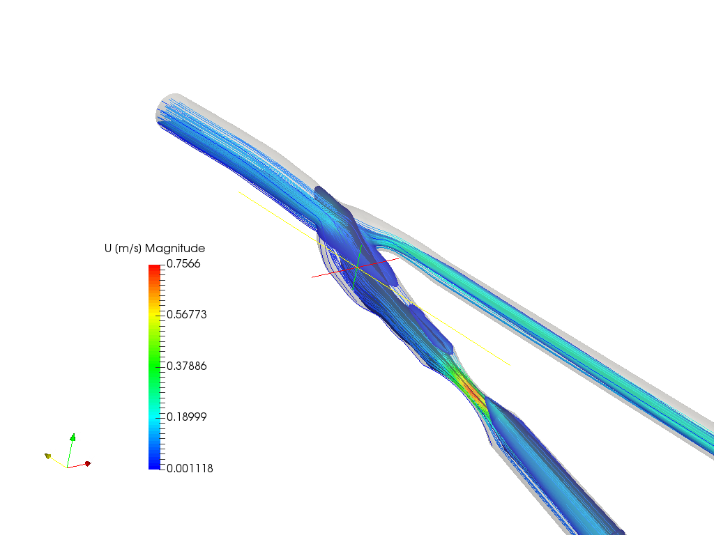
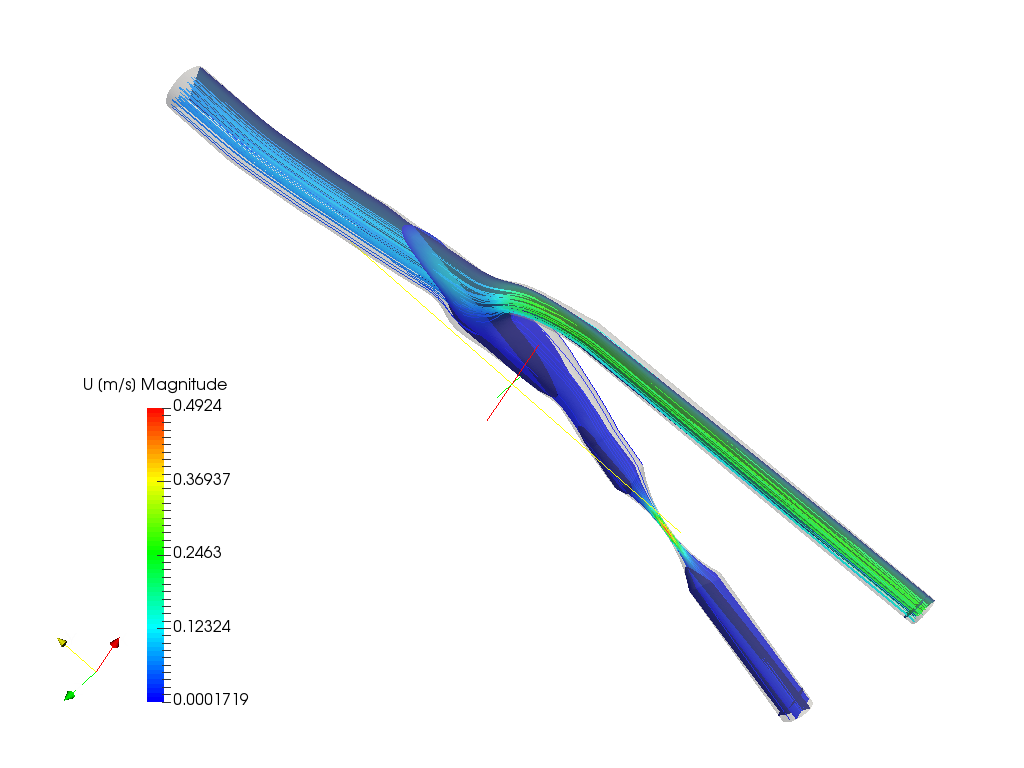
Then from the fields drop down (top-left corner) select U [point-data] to view velocity magnitude.
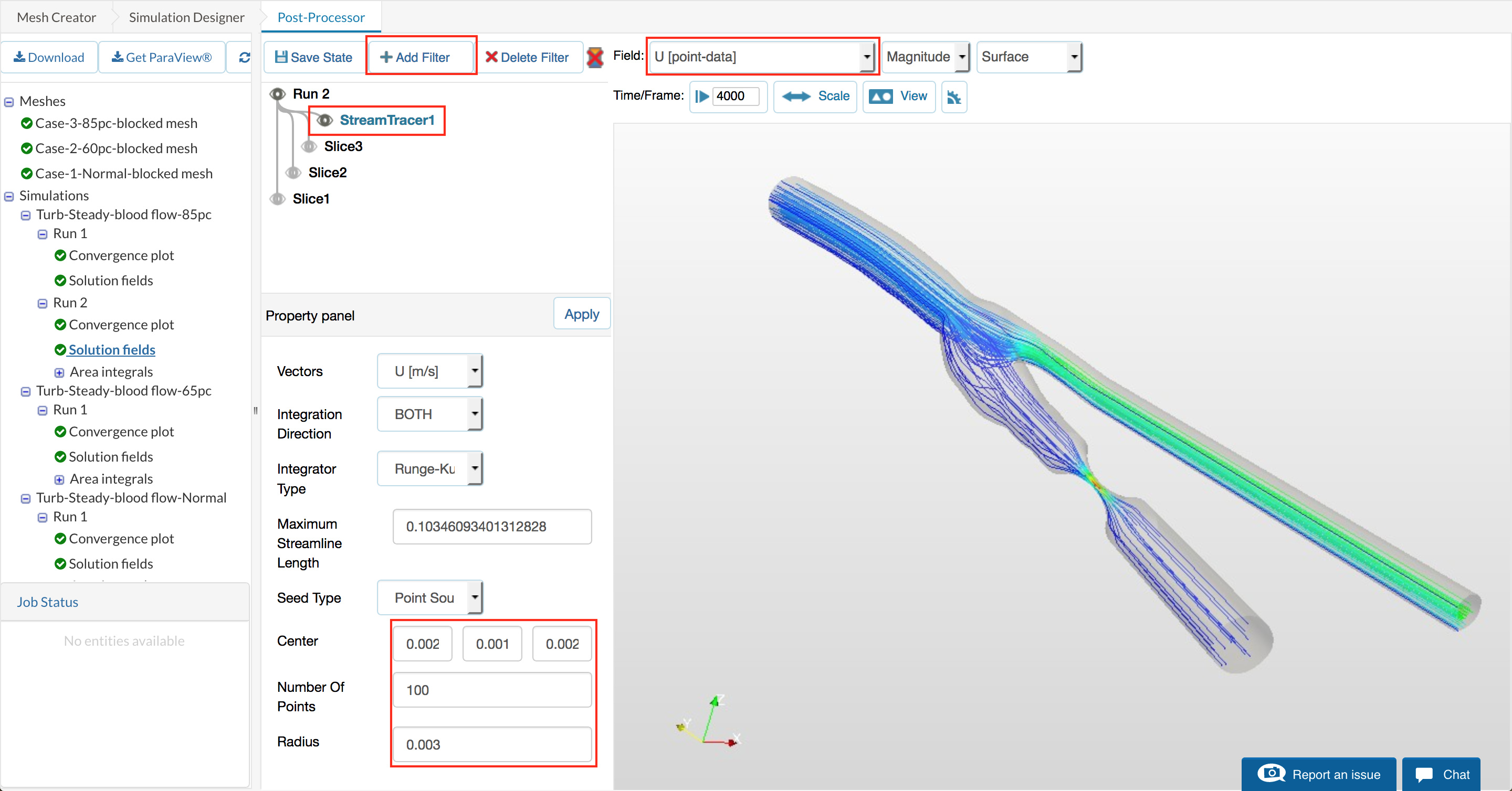
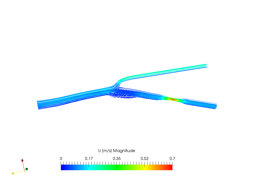
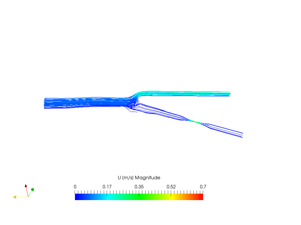
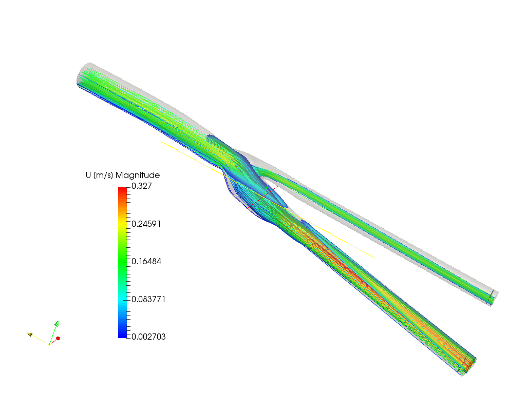
Figure 47: Shows streamlines of velocity vectors coloured by velocity magnitude.
Compare the results from each configuration, what observations can you make?
Comparing Viscosity
To observe how viscosity is affected by the blockages, it is useful to compare the results side by side. This can be done easily in the online post-processor adding additional solutions to the view and transforming them.
Start by adding the solution for the 85pc blocked case, do this by selecting the solution fields.
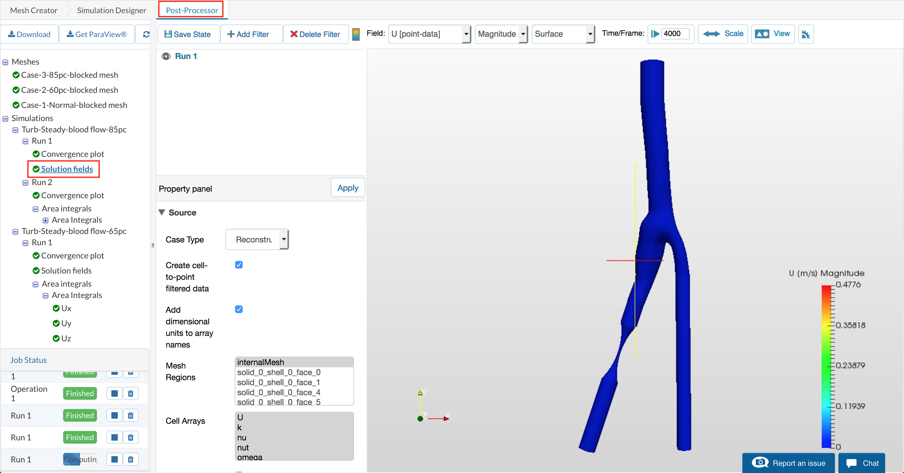
Figure 48: Bring a solution of case 3 - 85pc into the Post-processing viewer.
Once it is in the viewer, add a slice that is identical in setup to the previously defined Slice 1.
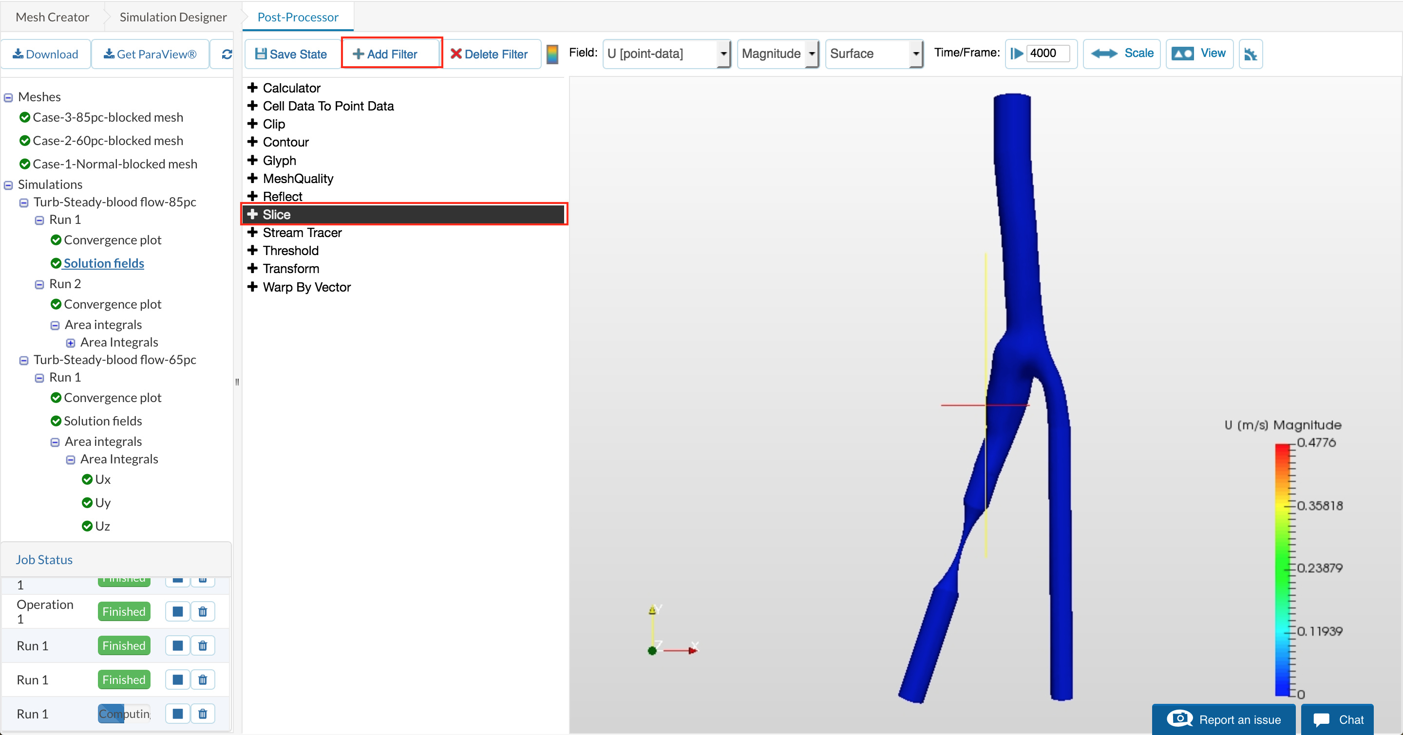
Figure 49: Add a slice filter.
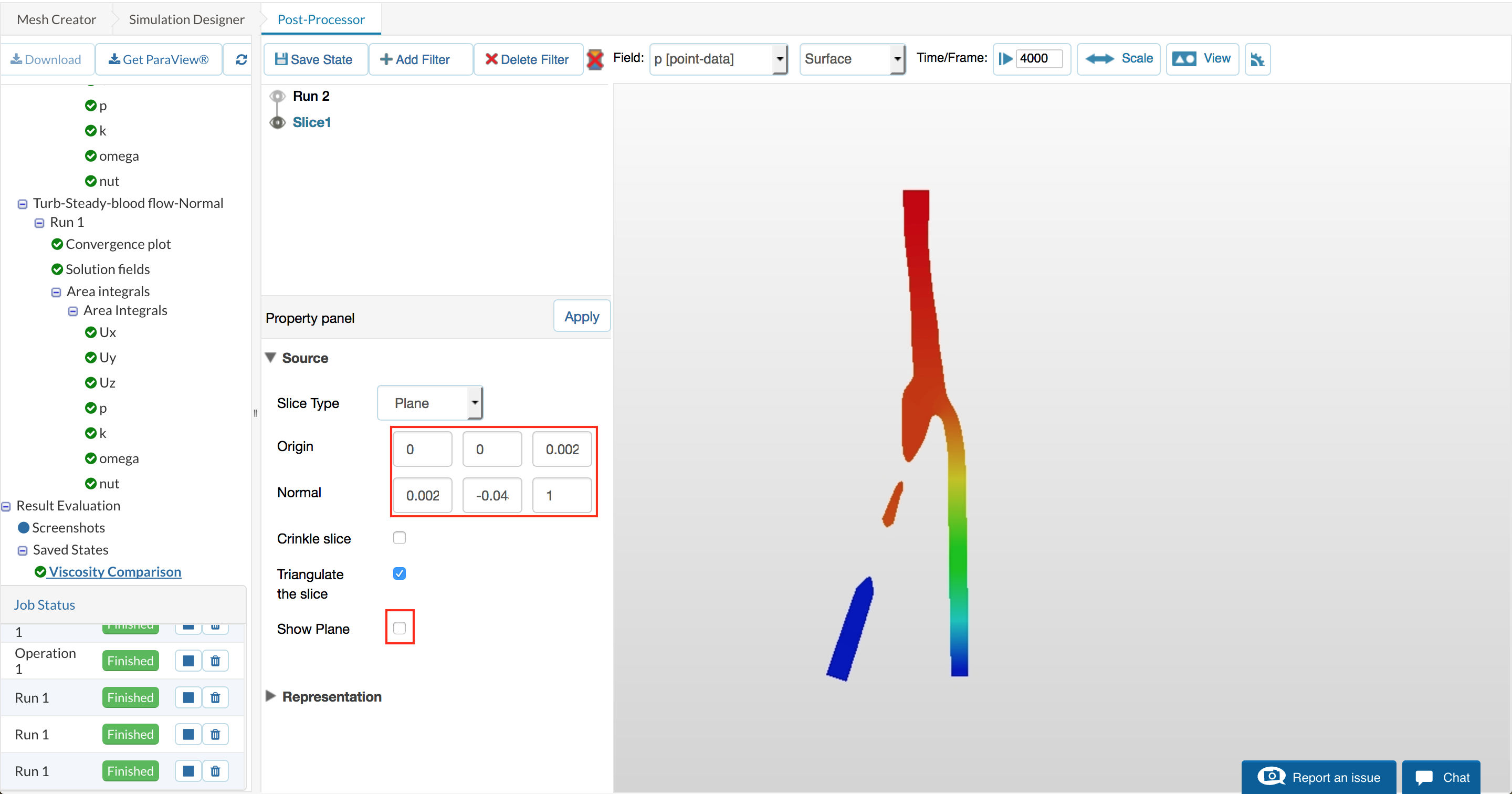
Figure 50: Change settings to those of slice 1 as was previously detailed.
Since viscosity is the field of interest this time, change the displayed field to nu.
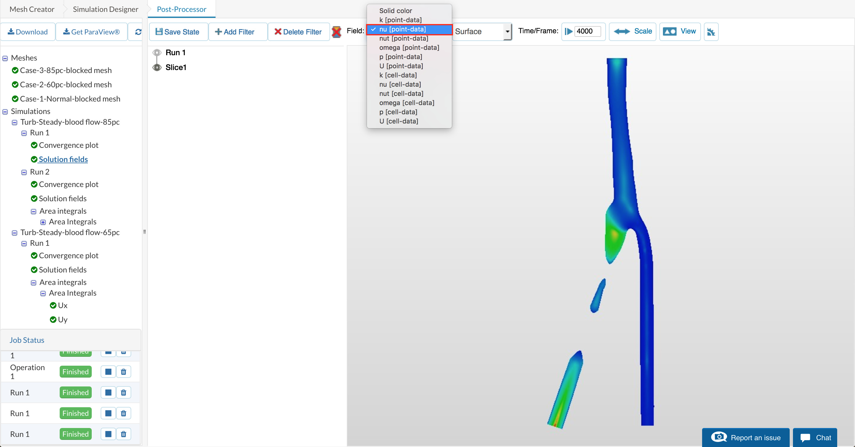
Figure 51: Change the coloured field to be viscosity (nu).
Now an additional solution needs to be added, this time instead of clicking the solution field of the 65pc case, right click and add it to the viewer. You should now see both solutions in the same Post-Processing instance.
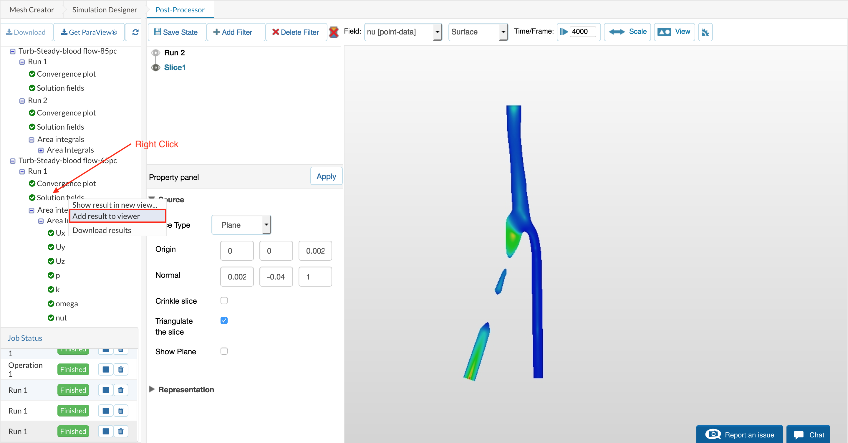
Figure 52: Bring in additional solution from case 2 - 65pc by right-clicking and adding to viewer.
Now add to that new solution the same slice as defined before. Change the display field once again to viscosity.
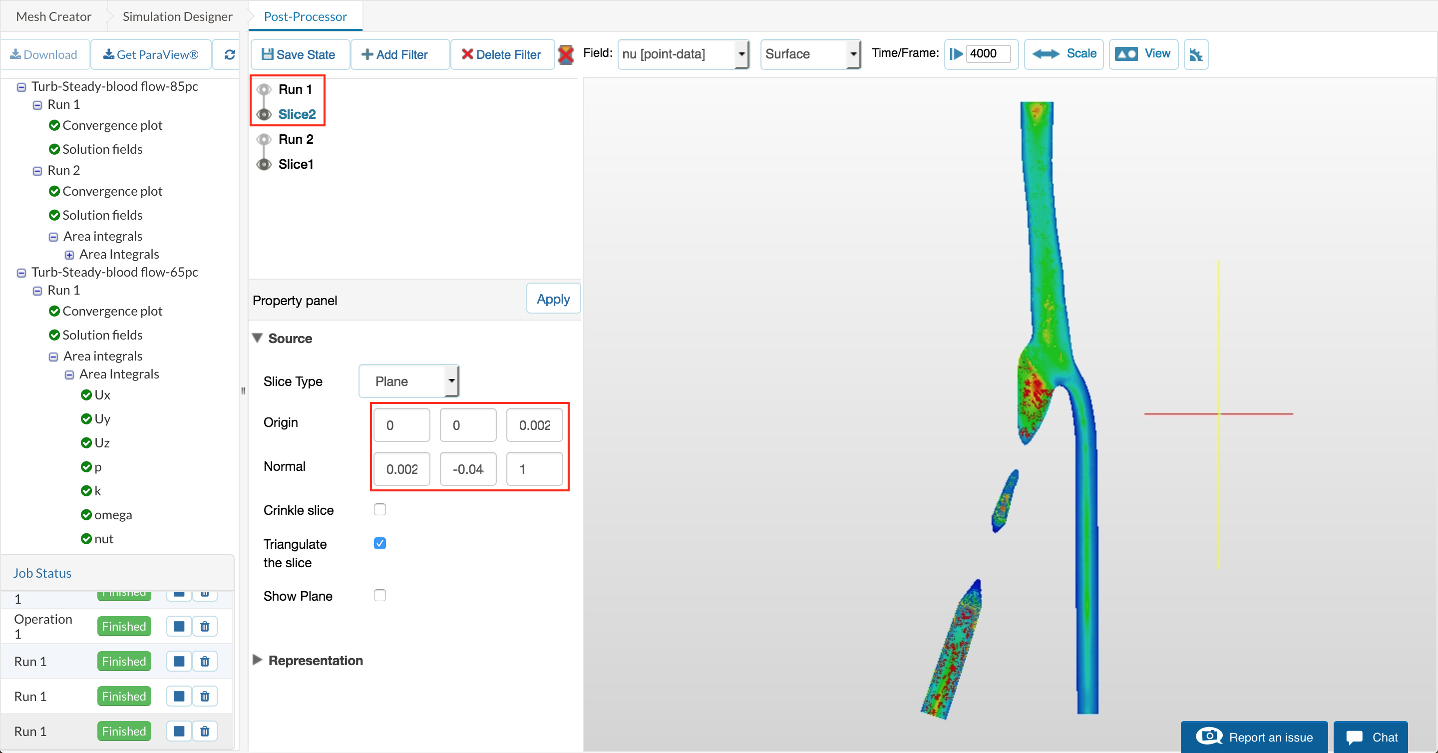
Figure 53: Add the same slice to the new solution.
Now we will add a new filter, transform moves the selected data in any direction, rotation or scaling. This is useful to reposition our results. Displace the results in the positive x-direction by 0.035m.
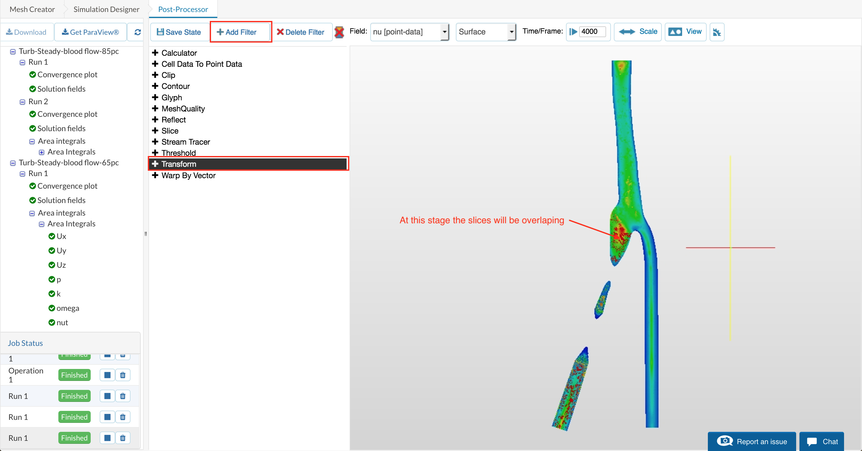
Figure 54: Add a transform filter to the new slice to display the solutions side-by-side.
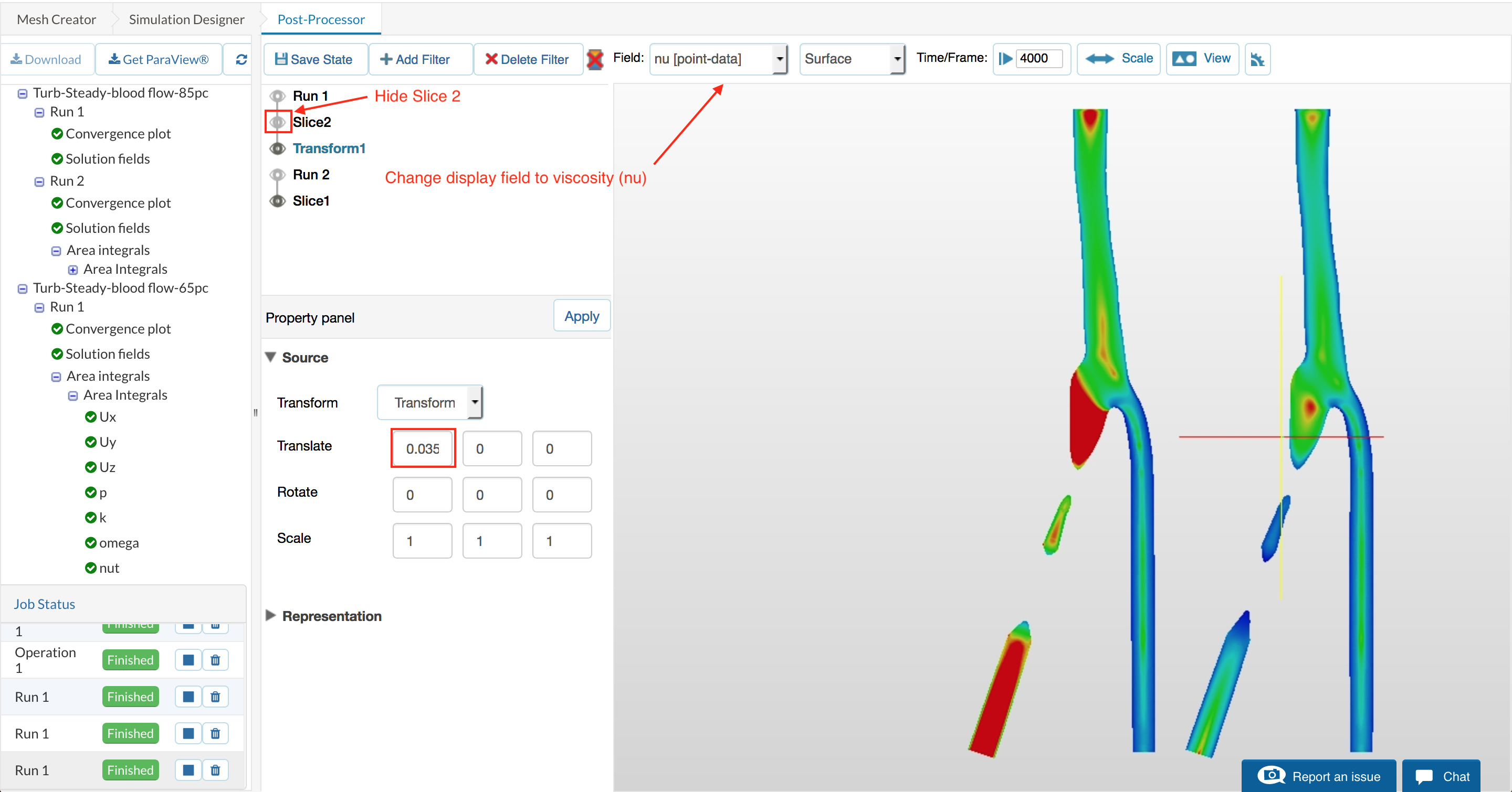
Figure 55: Transform the solution in the x direction by 0.035m.
Do the above steps for the final solution for the normal artery without blockages, but this time displace it in the x-direction by 0.07m. This will show all solutions next to each other.
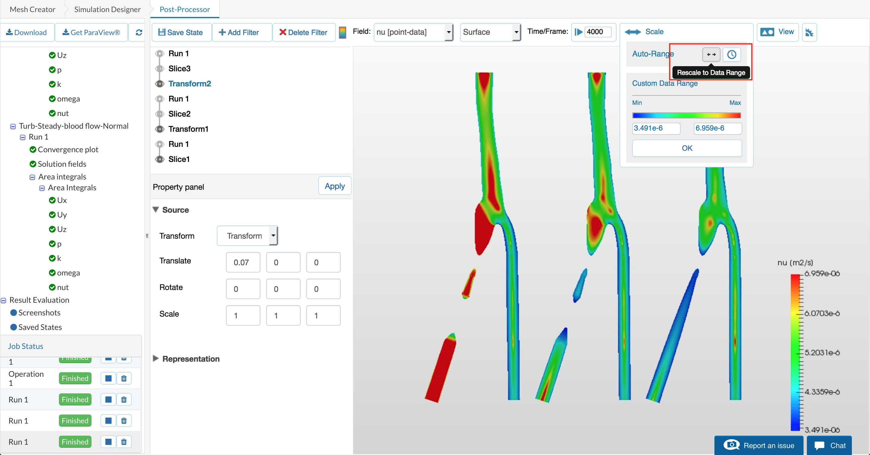
Figure 56: Rescale viscosity to the visible range.
Finally, we can save this state so that it can be re-used at a later date by clicking the Add State button, and a Post-Processing image can be created from the viewer by navigating to View and then clicking the image capture button.
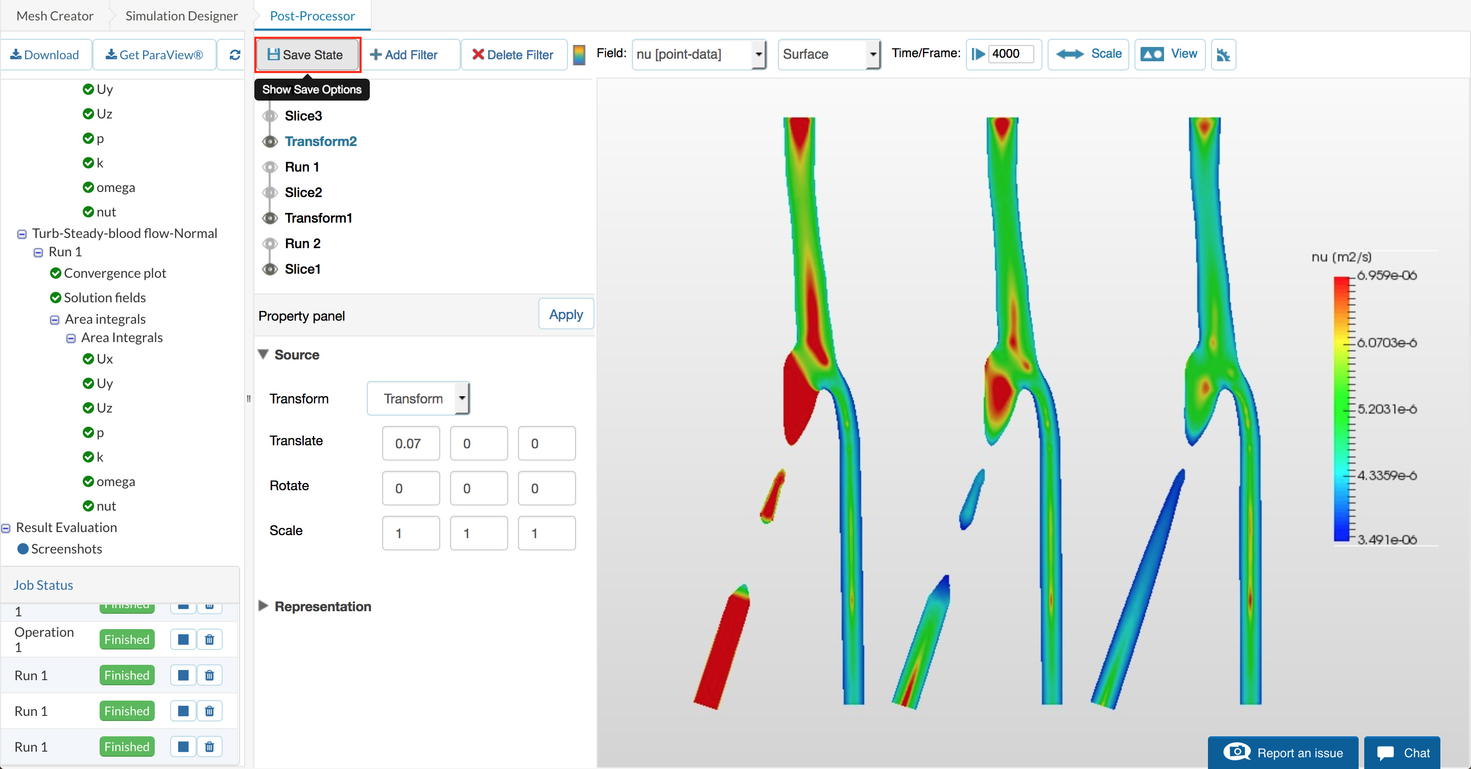
_Figure 57: Displays all solutions side-by-side, save this sate with the save state button.
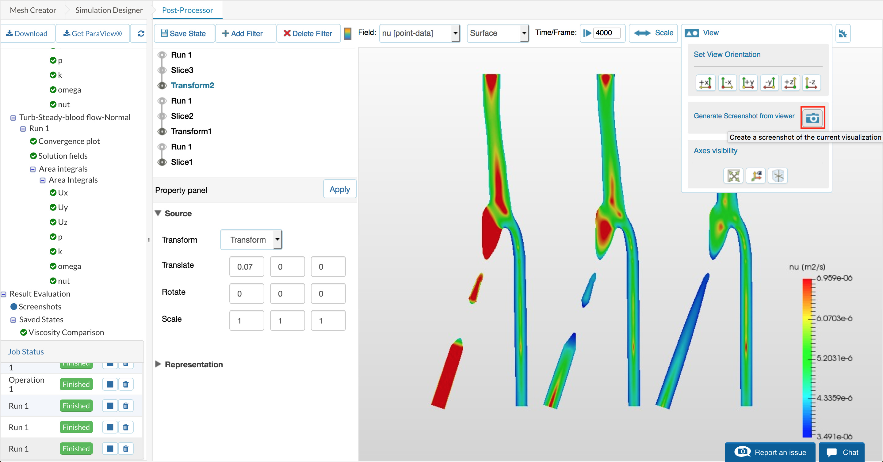
Figure 58: Save screenshot of the Post-Processing views.
What do these results say about viscosity in each of the cases? and how might this further affect the patient’s health?
Viewing Result Control Items
In the Post-Processor under the simulation run, there will be an area average item expand it and expanded the integral node also. View the integral for Uy, this represents the volume flow rate. Compare the final value to the other simulation runs.
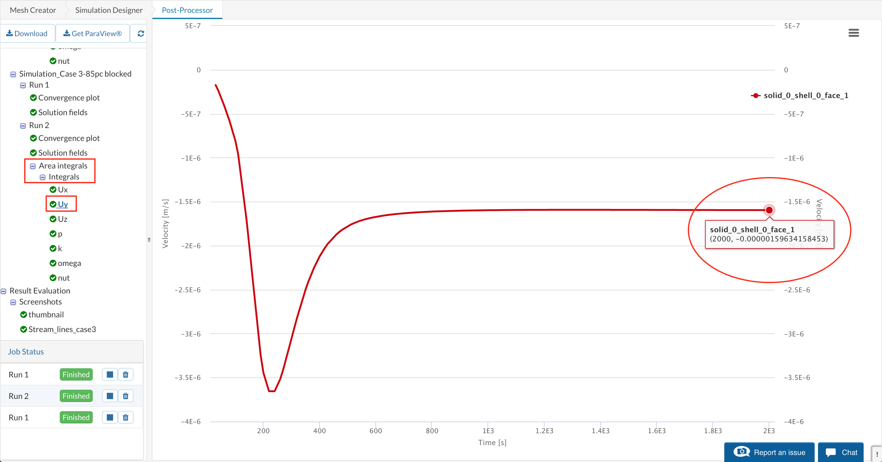
_Figure 59: Integration Plot for velocity in the y direction, representing volume flow rate during the solution.
We can quickly create a plot from these values to compare the flow rates between the healthy and blocked arteries.
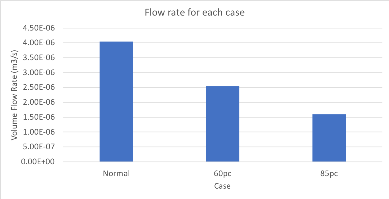
Plot 1: Shows the flow rates due to the defined pressure differences for each case.
What does this mean for health of the patient?
References
[1] The base CAD model for the Artery used in this homework session is provided by aaron from GrabCAD . It was modified and prepared for CFD analysis.