Recording

Homework submission
Submitting all three homework assignments will qualify you for a free Professional Training (value of 500€) as well as a certificate of participation.
Homework 1 - Deadline 21.07 12:00pm
Exercise
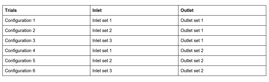
This exercise involves simulating the ventilation inside an aircraft cabin. For simplicity and reduced computation there is only one row of seats in the geometry. The task is quite interesting, to setup 6 different configurations by having various configurations of inlet and outlet, and then to compare the results. The possible inlets and outlets are as shown in the following figure.

The different combinations for performing the simulations are
Step-by-Step
Import the project by clicking the link below. ( Crtl + Click to open in a new tab )
Click to Import the Homework Project
Once the project is imported, the workbench is automatically opened. Then follow the steps below for setting up an incompressible flow simulation.
Meshing
- In the ‘Mesh Creator’ tab, click on the geometry ‘Aircraft cabin’
- Then, click on ‘New Mesh’ button in the options panel.

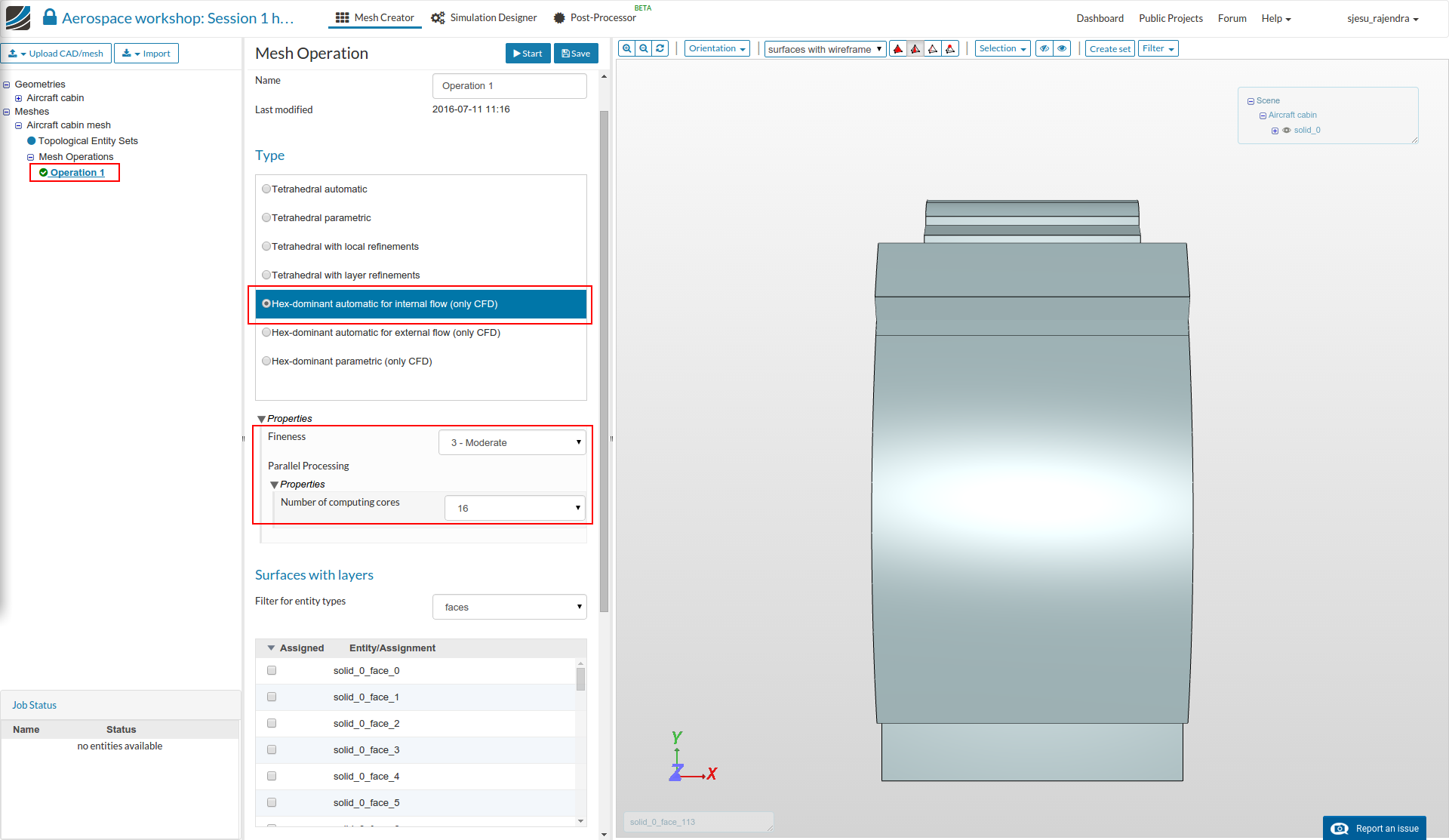
- Select Hex-dominant automatic for internal flow (only CFD) mesh and select the following parameters - Moderate fineness and 8 cores. This operation will automatically create a mesh for fluid flow simulation. The cell size and refinement will be adapted automatically.
- Since this is expected to be a turbulent flow, layers are required for all the faces except the symmetry walls. Prism layer cells are characterized by very flat elements that are able to resolve the boundary layer appropriately.
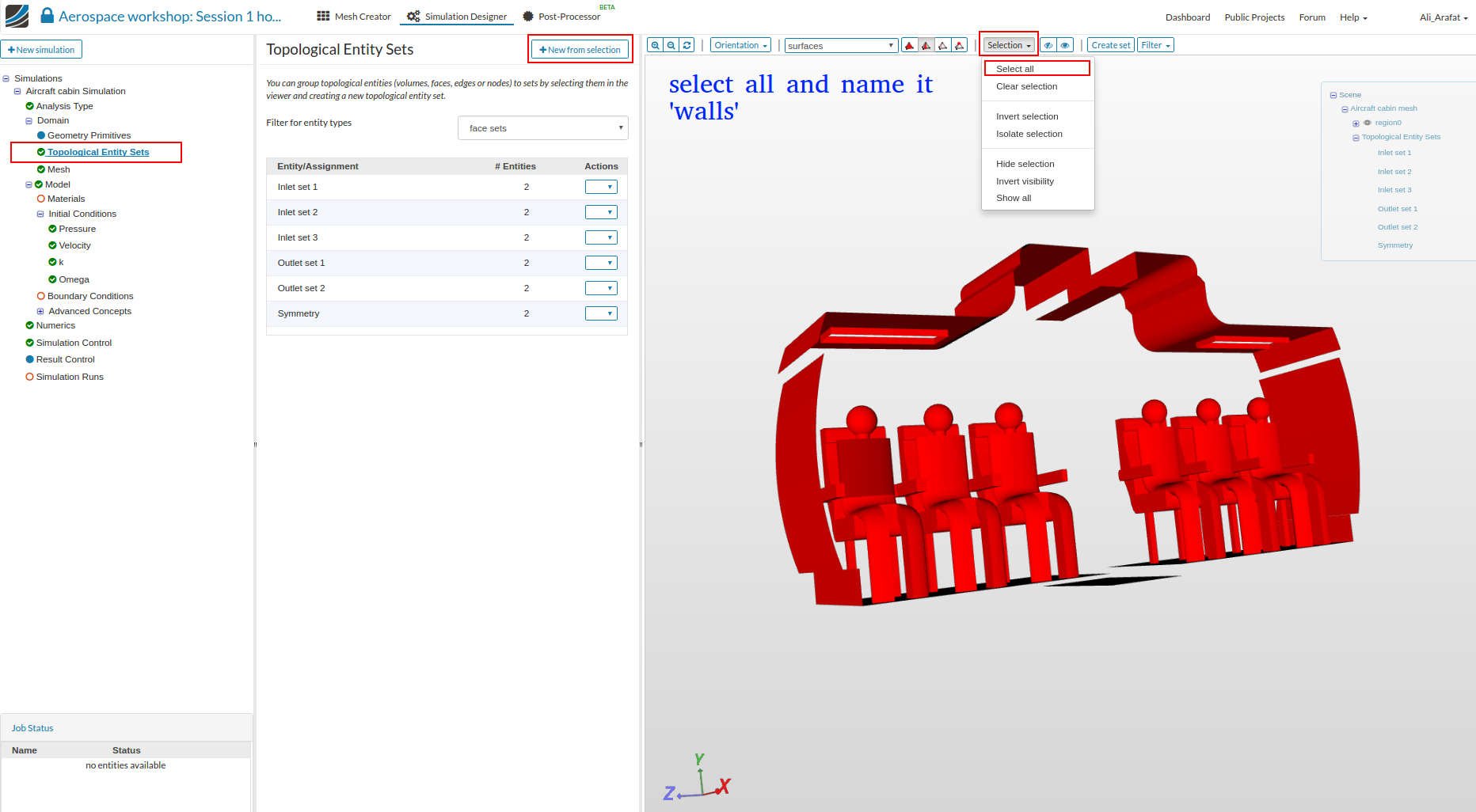
- First click the ‘Selection’ drop down list from the tool bar and click on ‘Select all’
- Then click the 2 symmetry faces to de-select them.

- Click the Add selection from viewer button [1] and select Save [2].
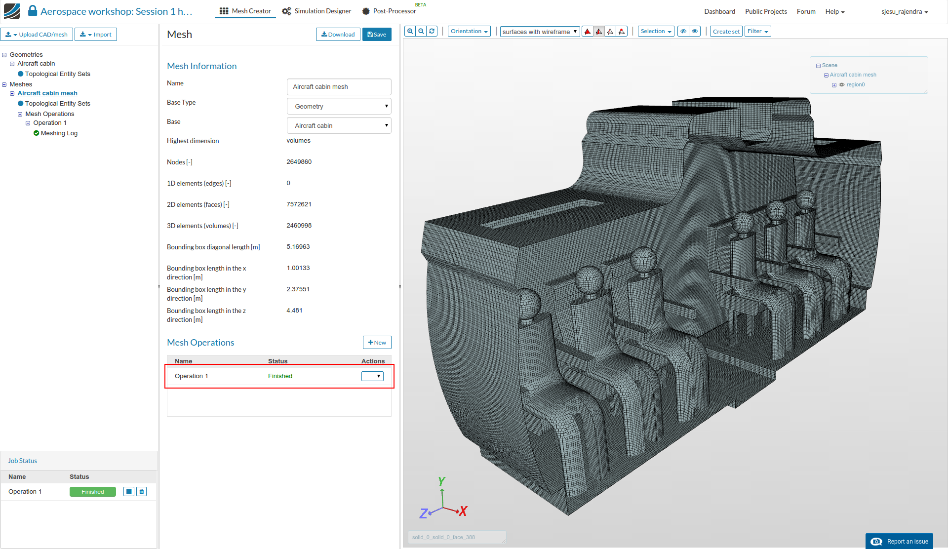
- Now click the Start button [3] to begin the mesh operation. The meshing job will start in a few moments and all computation is done via cloud computing.

- The mesh operation takes about 15 minutes to complete and gives a ‘Finished’ status in the lower left once it is over.
Simulation Setup
- For setting up the simulation switch to the Simulation Designer tab and select New simulation.

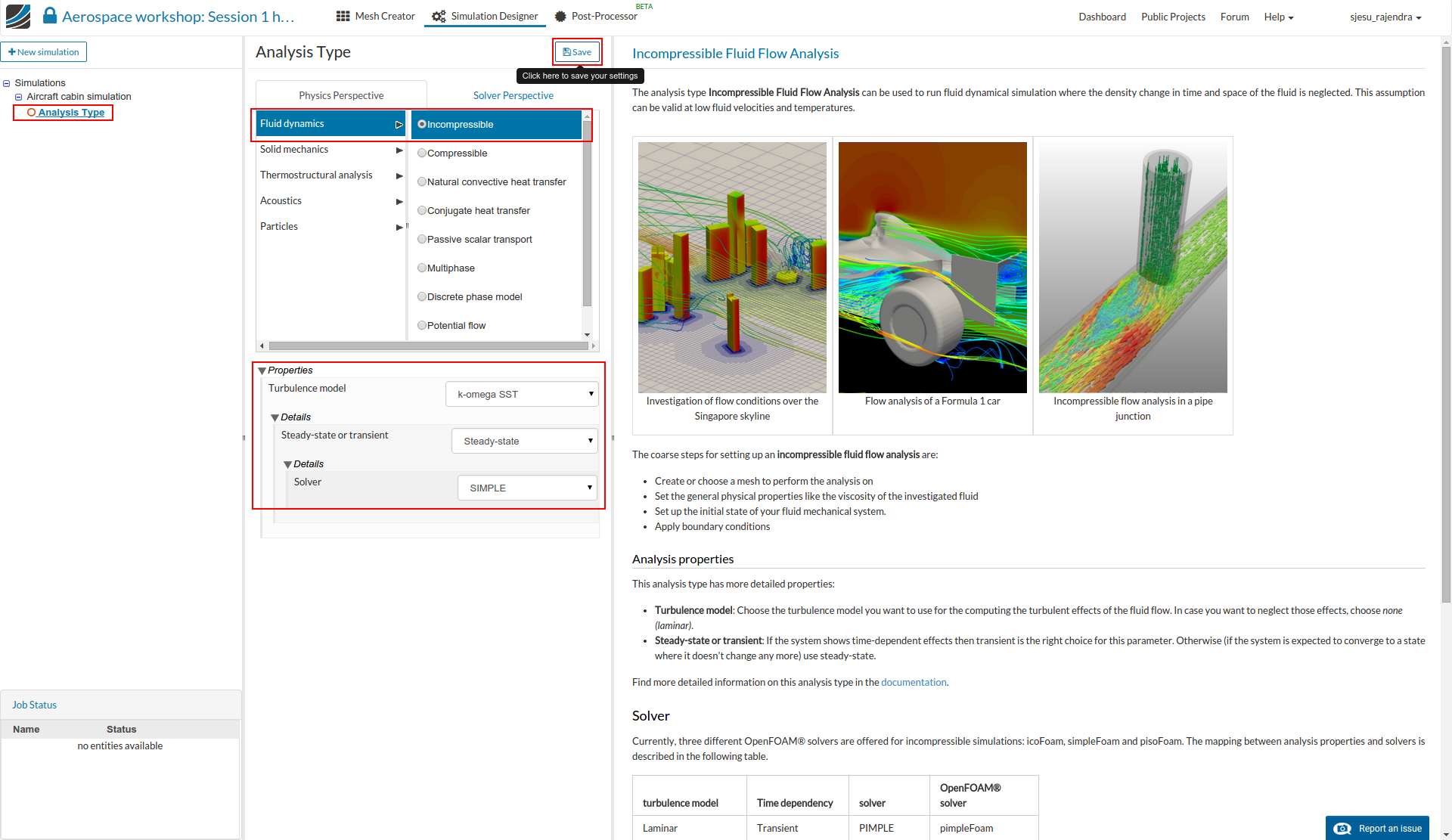
- Select the analysis type: Incompressible under Fluid dynamics.
- Select k-omega SST as the turbulence model and Steady-state type and click Save button.
- The flow in aircraft cabin is assumed to be Incompressible due to low velocities of the circulated air. Choosing Steady-State option means that we will simulate the Time-Independent solution.
- After saving, the simulation tree now looks as shown below. Here the Tree Entries in Red must be completed.

Domain selection
- Click ‘Domain’ from the tree and select the mesh created from the previous task. Click the Save button. The mesh will then automatically load in the viewer.

Create Topological Entity Sets
- In this homework we are going to perform 6 different simulations, as discussed earlier. The image below shows various settings for inlet and outlets. It is convenient to name these under ‘Topological Entity Sets’ to be used later during the setup.
- We will create 7 sets in total, as shown below:
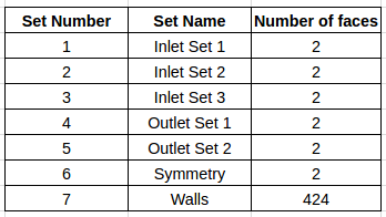
- Click on the tree entry ‘Topological Entity Sets’.
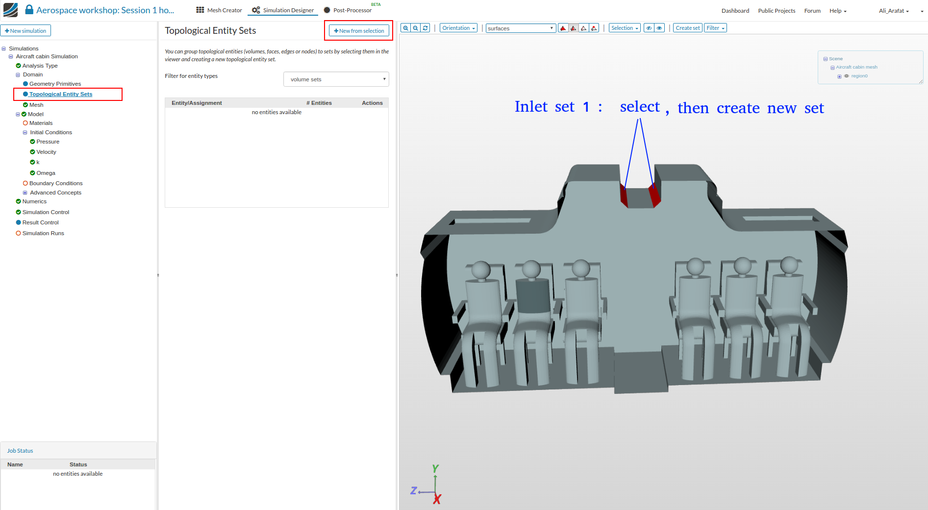
Inlet Set 1:
- To create the first set, click the shown surfaces and click on the ‘New from selection’ button to create a set named ‘Inlet Set 1’.
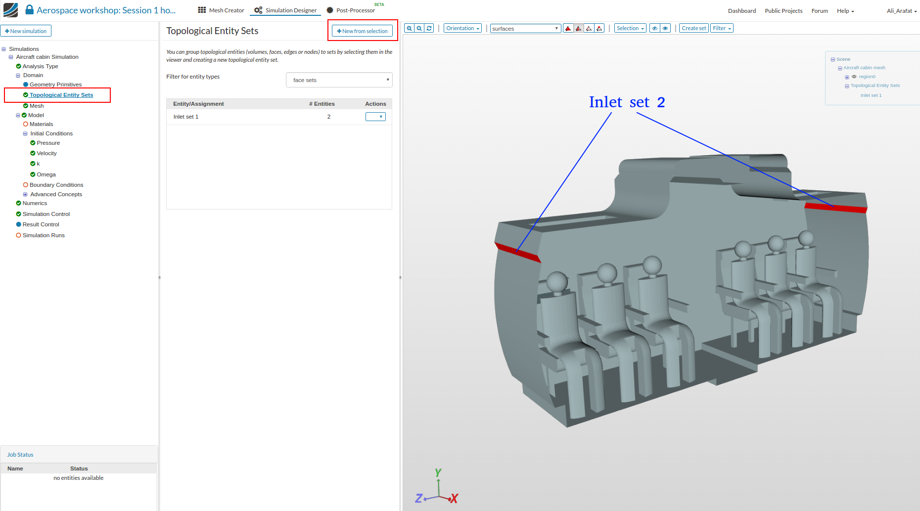
Inlet Set 2:
- Similarly, select the shown surfaces and create a new set named ‘Inlet Set 2’.
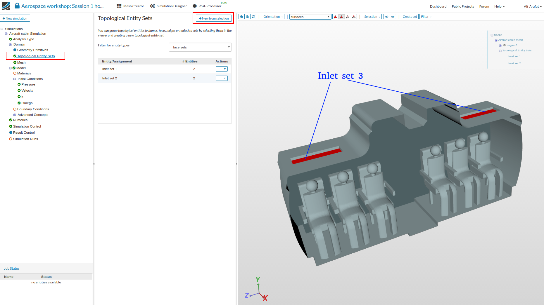
Inlet Set 3:
- and then the shown surfaces for the third inlet set.
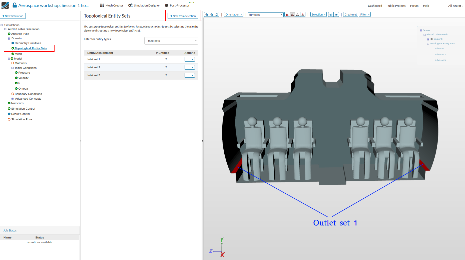
Outlet Set 1:
- For the outlets, select the shown surfaces and click ‘New from selection’ button to create a set named ‘Outlet Set 1’.
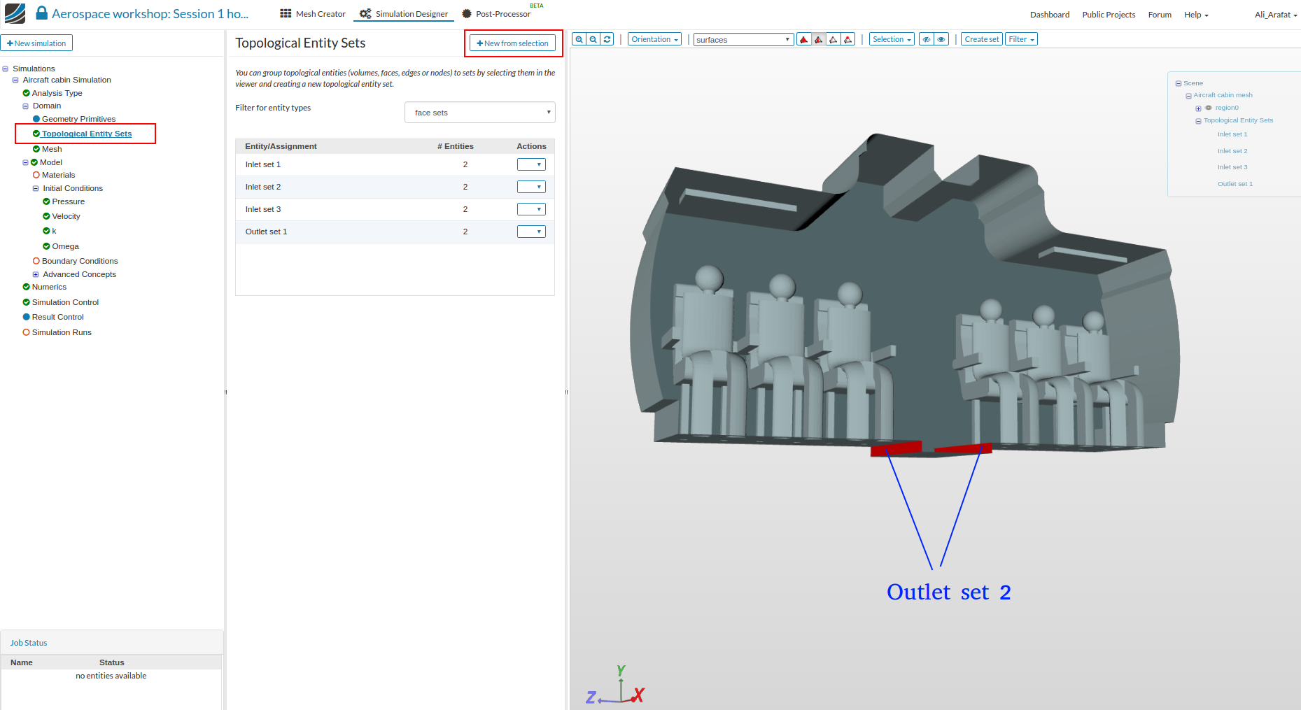
Outlet Set 2:
- Similarly for the second outlet set.
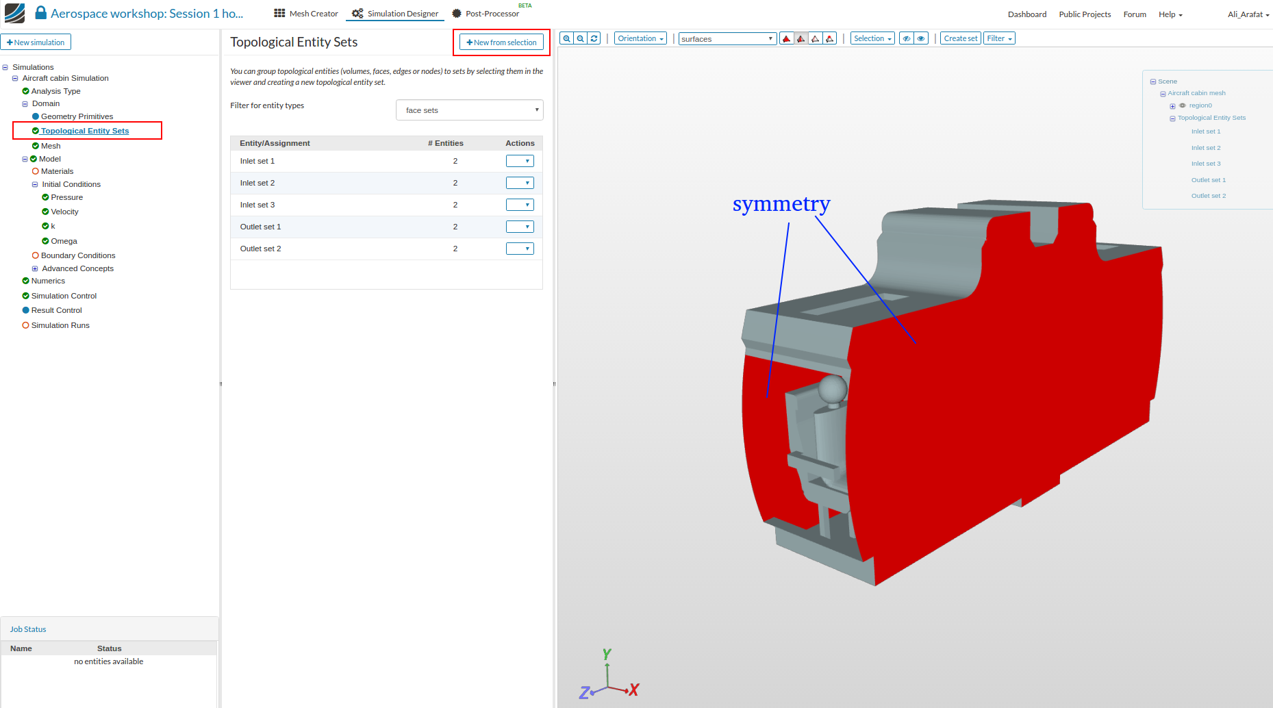
Symmetry:
- Select the shown faces and create a set named ‘Symmetry’.
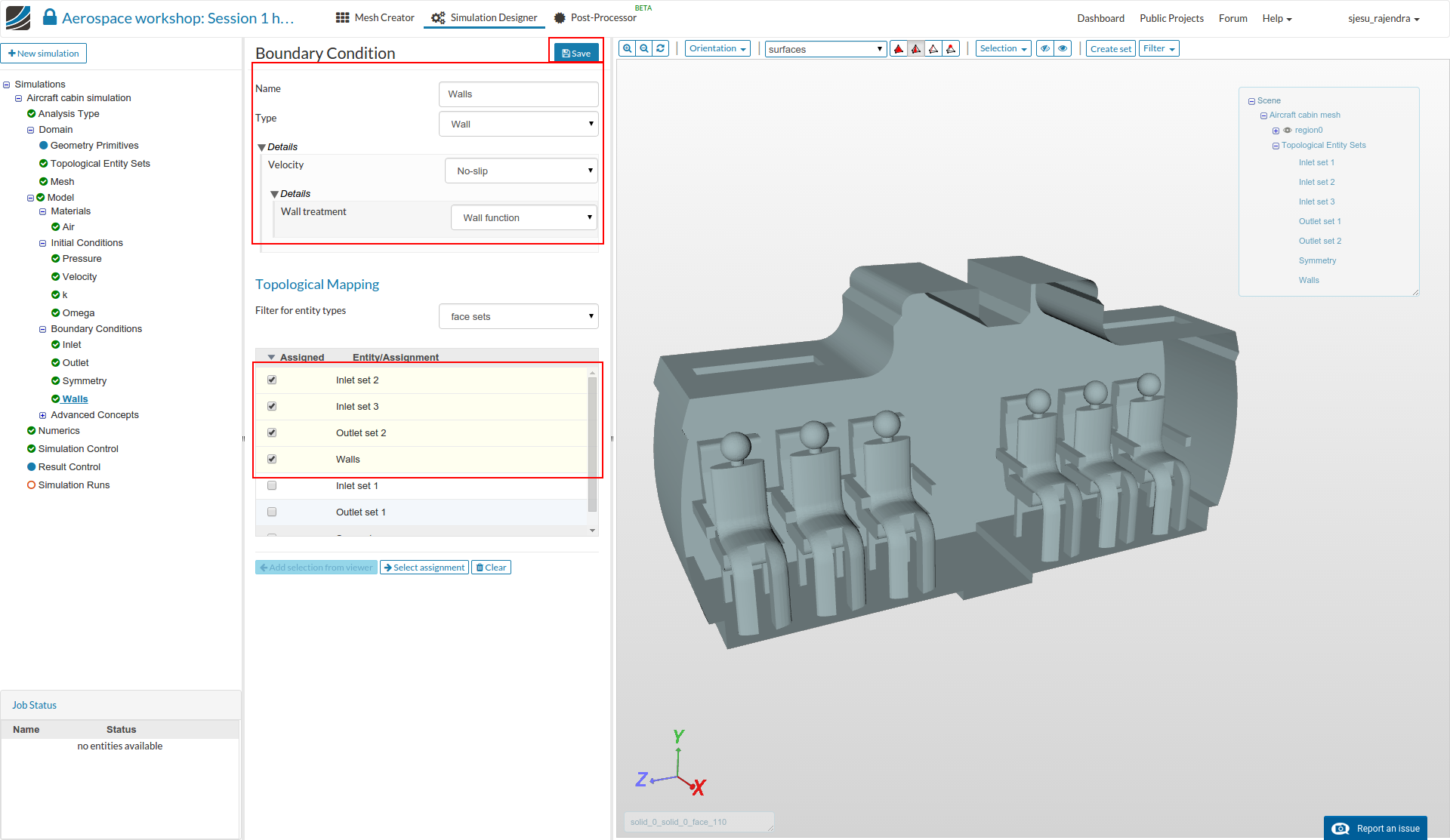
Walls:
- Now select each created set and hide it from the viewer, as shown in the image below. This would enable us to select all the remaining faces as ‘Walls’.
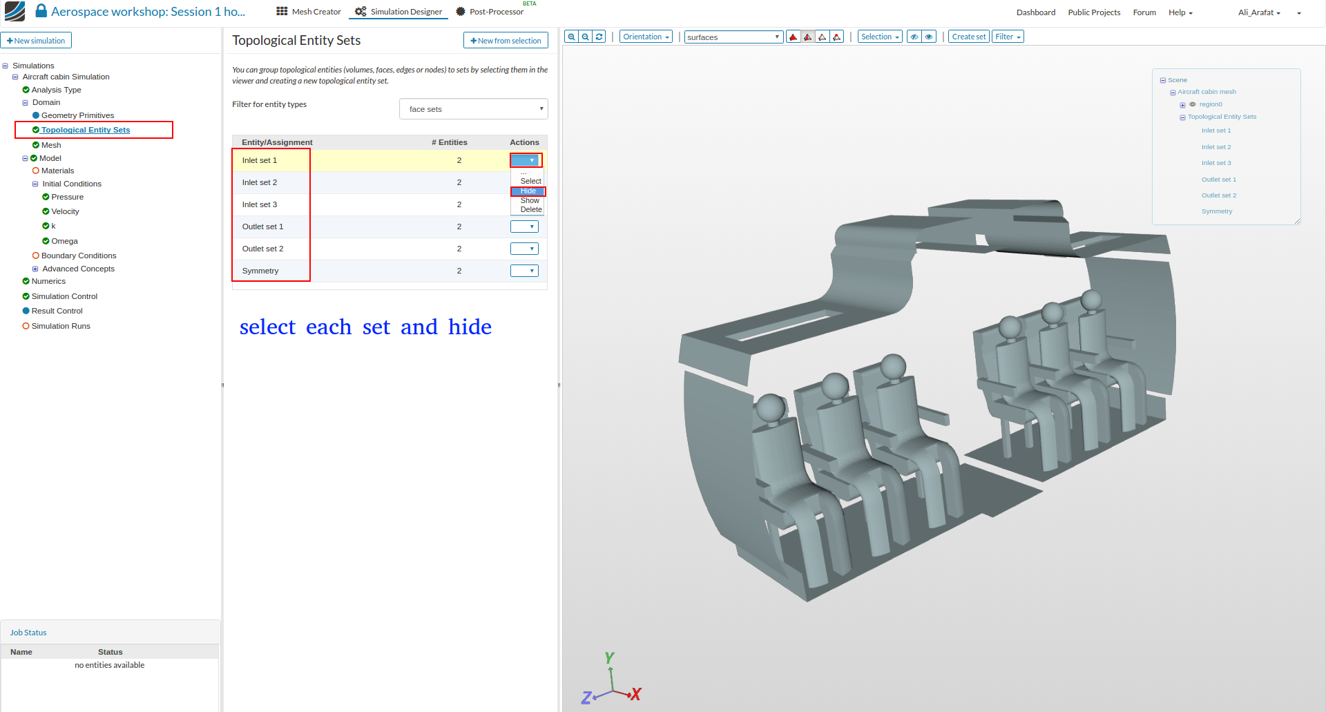
- From the toolbar click on ‘selection’ and click ‘Select all’. Then create the last set and name it as Walls.
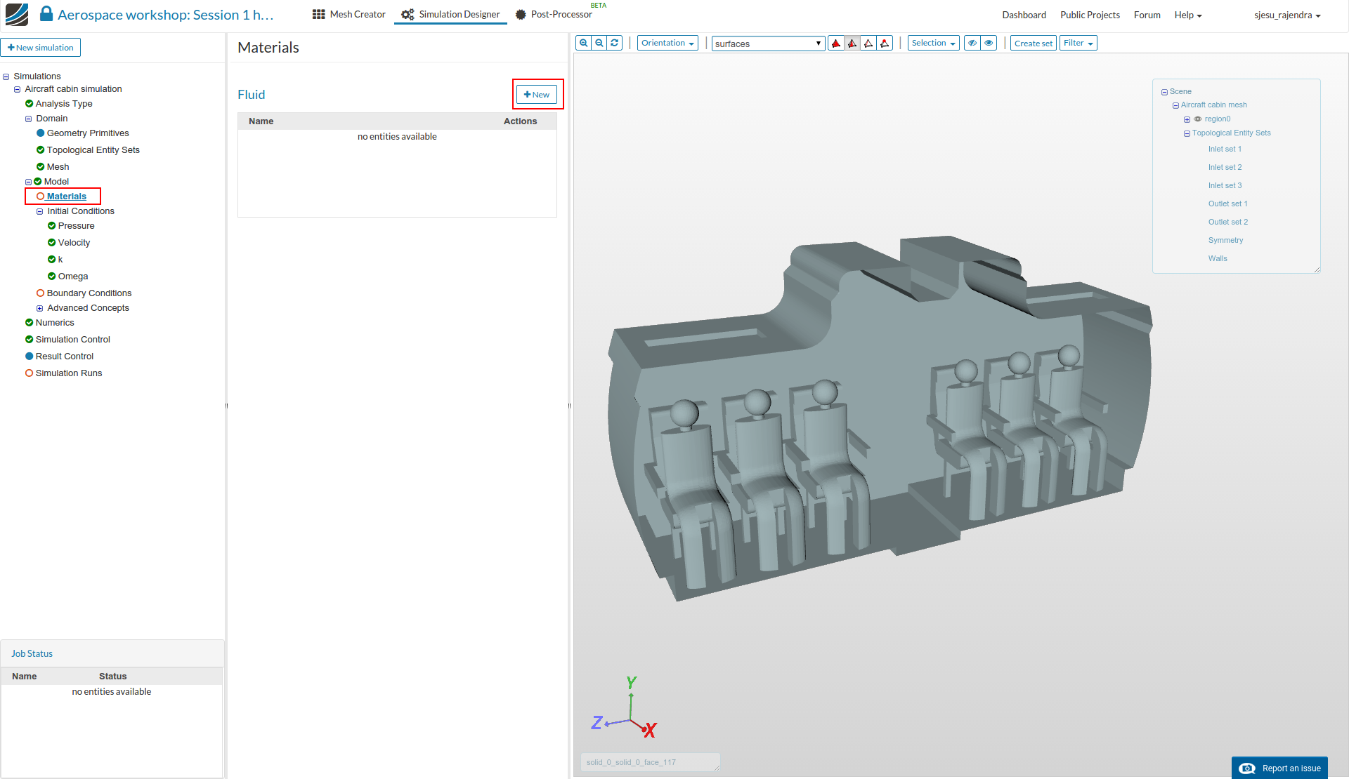
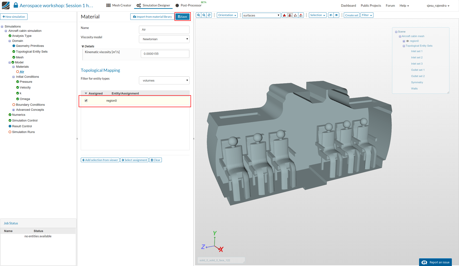
Select Fluid Material
- Select ‘Material’ from the sub-tree and click New.
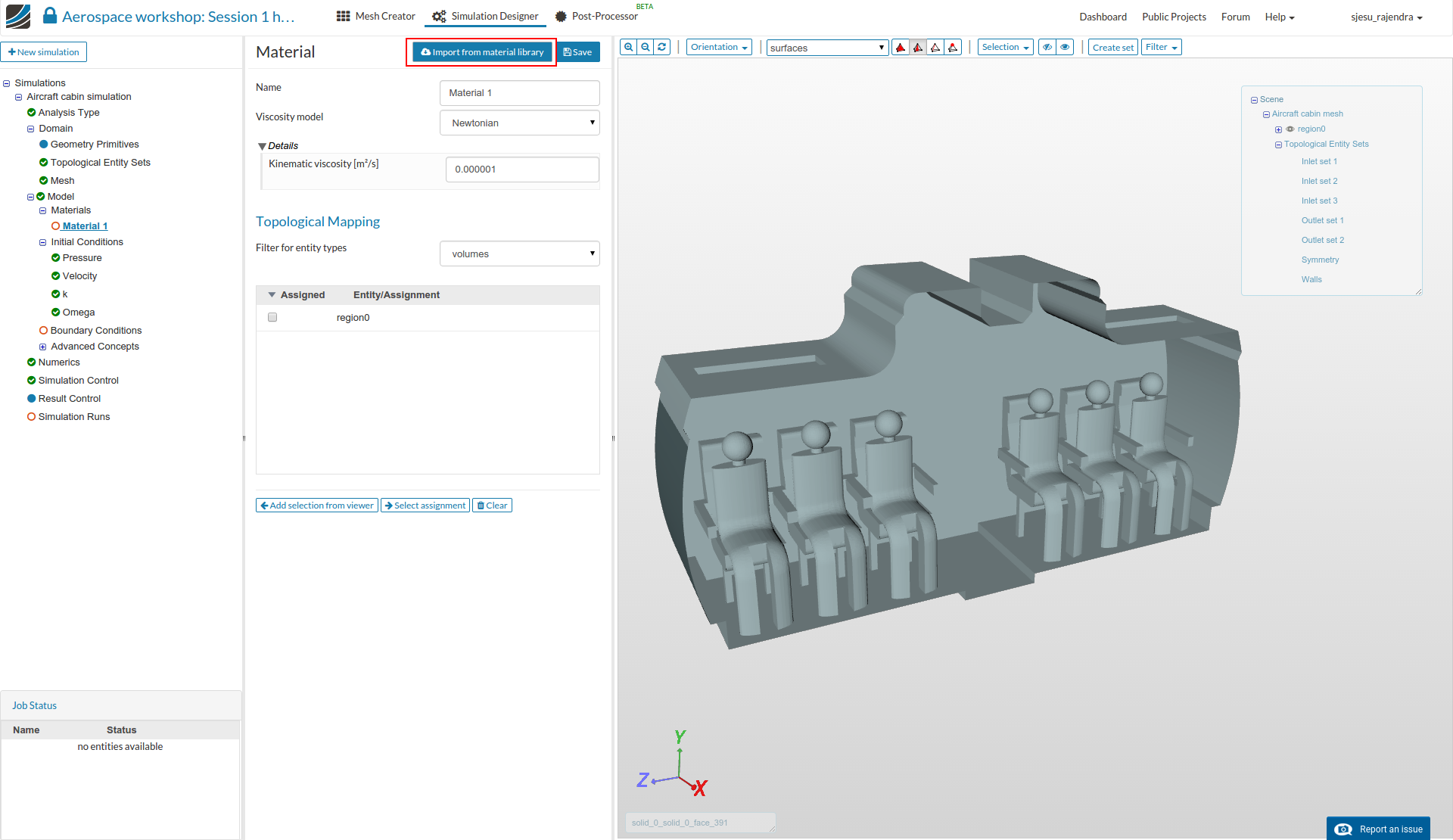
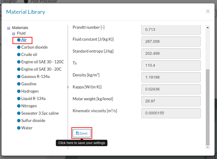
- Select Import from material library in the top of the pane.
- Click Air and select the Save button.
- Select region0 from Topological Mapping and click the Save button.
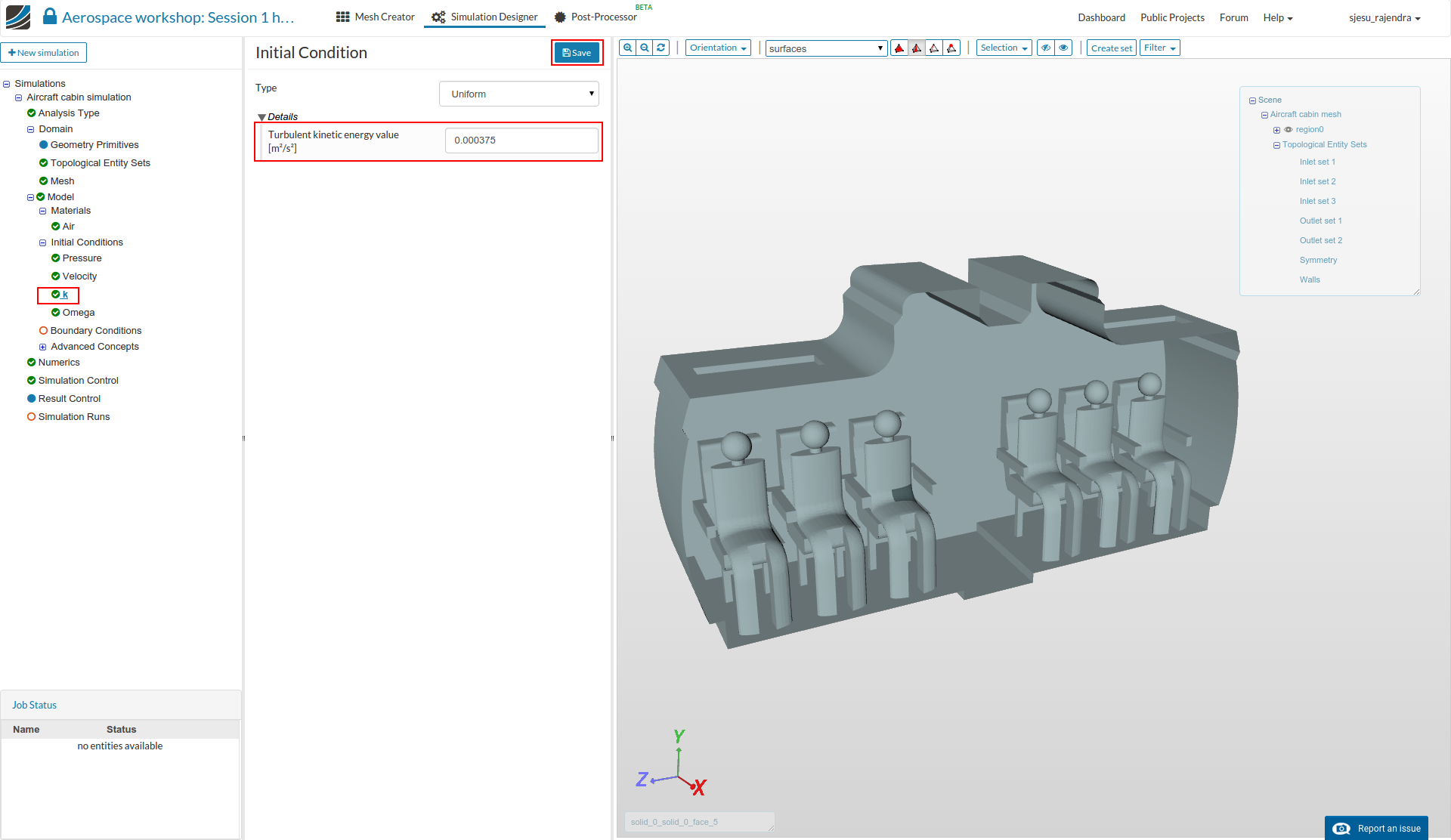
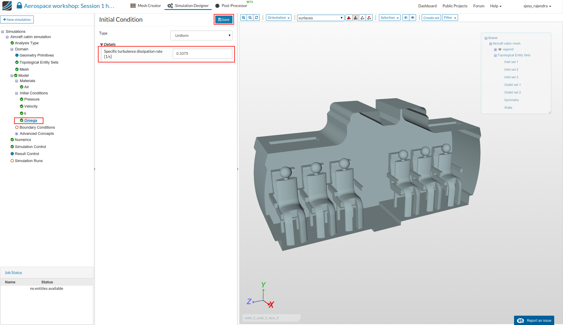
Initial Conditions
- Under ‘Initial condition’ from the tree, select k and Omega and enter the values as shown in the following figures. Click the Save button everytime.
Boundary Conditions
The boundary conditions define the flow variables at the boundary surfaces.
- Click on ‘Boundary condition’ and select New.

Inlet :
- Enter the inlet boundary condition with a volume flow rate of 0.02975 cu.m/s. Select the Inlet set 1 entity and click Save option.

- The inlet volume flow rate for Configuration 3 and 6 are maintained to be 0.07105 cu.m/s. The values are calculated such that a velocity of 0.35m/s is obtained in all cases.
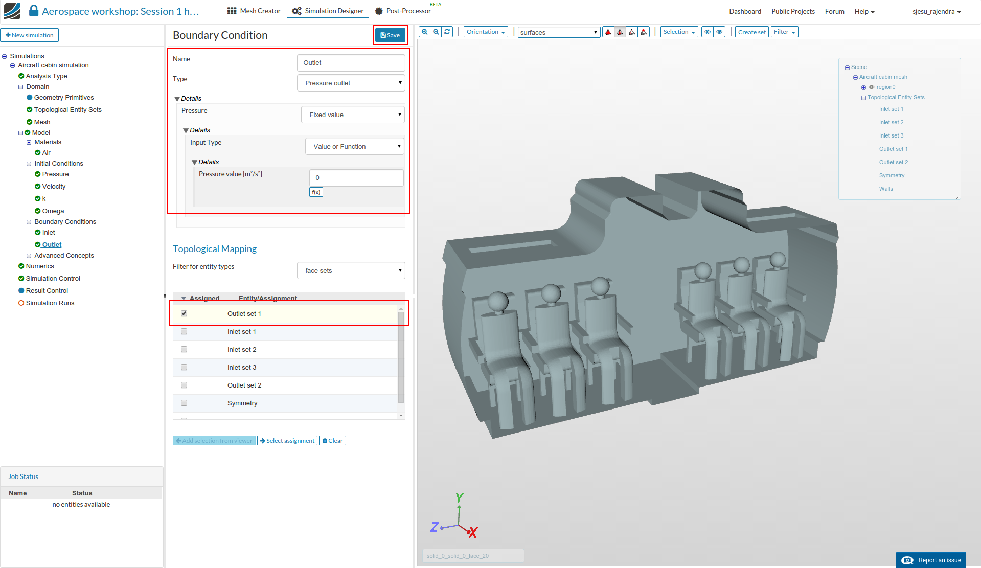
Outlet :
As the velocity is not known at the outlet faces, we would define the pressure here.
- Define a pressure outlet boundary condition to Outlet set 1 and click Save.
Symmetry :
- Next we will define the symmetry condition.

Walls :
-
The remaining boundary definition is for the walls. One important thing to be noted is that this condition has to be assigned to all entities which are not defined the previous 3 conditions.
-
Hence for Configuration-1 setup ‘Inlet set 2’, ‘Inlet set 3’ and ‘Outlet set 2’ are also considered as walls.
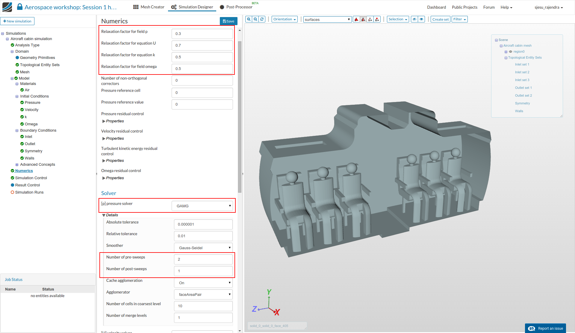
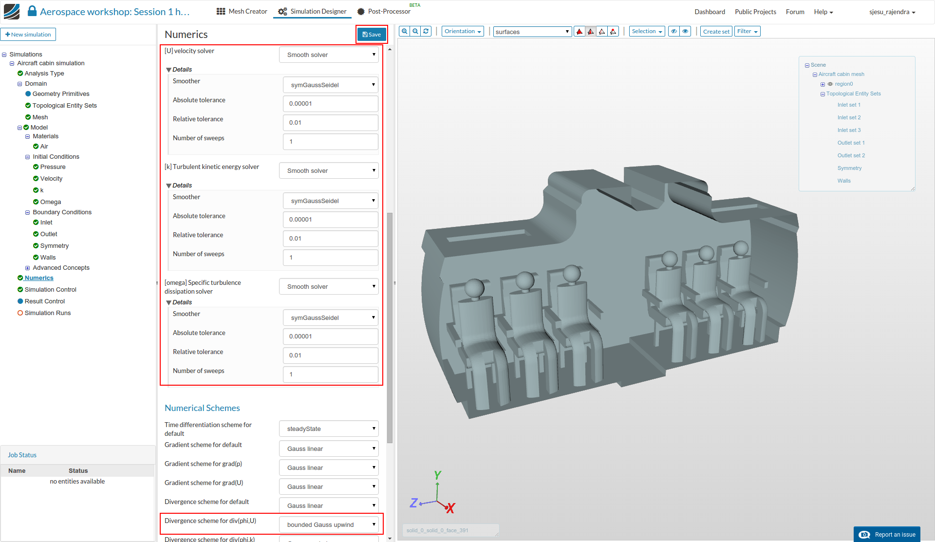
Numerics
-
Select ‘Numerics’ from the sub-tree and enter the following values. This enhances the solver to get the appropriate results.
-
Set the relaxation factors to:
P : 0.3
U : 0.7
k : 0.5
Omega : 0.5
-
Set ‘GAMG’ solver for pressure with 2 pre and 1 post sweep.
-
Set ‘Smooth Solver’ for the rest with the shown settings.
-
Set the ‘Numerical scheme’ for Div(Phi,U) to ‘bounded Gauss Upwind’
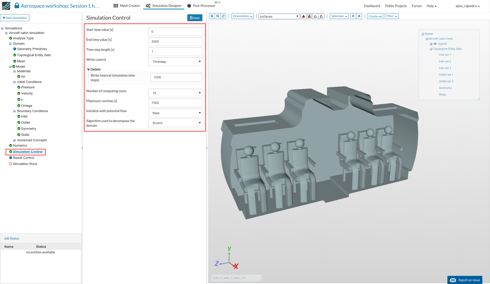
Simulation Control
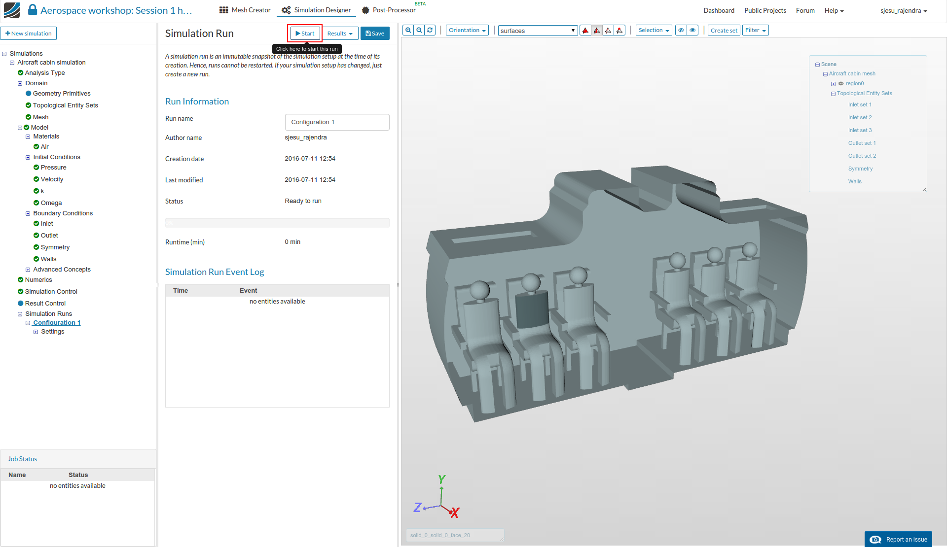
- Click on ‘Simulation control’ and setup the simulation run for 2000s time with a time step of 1.
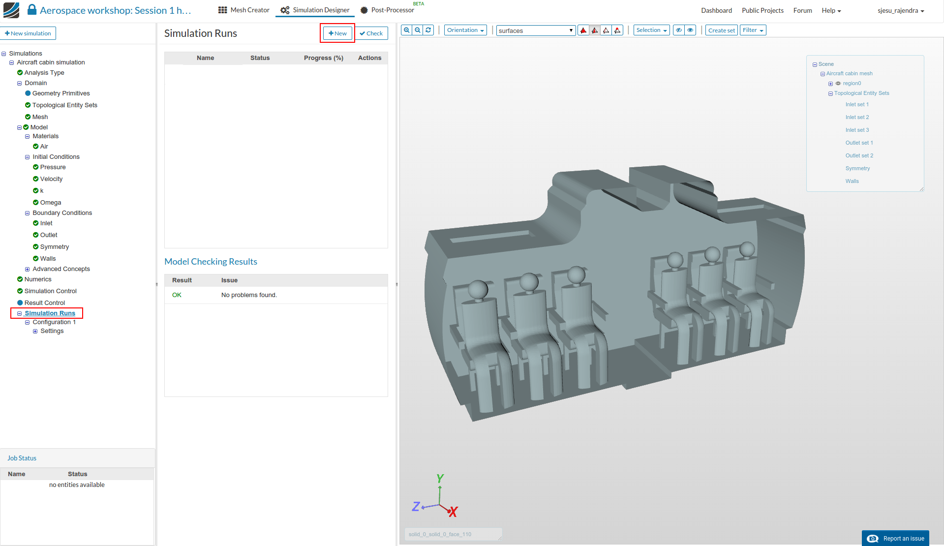
Create New Run
- Click on Simulation runs and create a new run.
.
Create Further Configurations
-
Similarly create 5 other configurations (2-6) with the following conditions.
-
You can ‘duplicate’ the previous simulation setup by right clicking and selecting duplicate. Then change the boundary conditions. Make sure not just to set the inlet and outlet conditions, but also the wall boundary condition assignments need to be changed (all the faces except inlet, outlet and symmetry) each time.
-
Only the Symmetry boundary condition assignment remains unchanged.

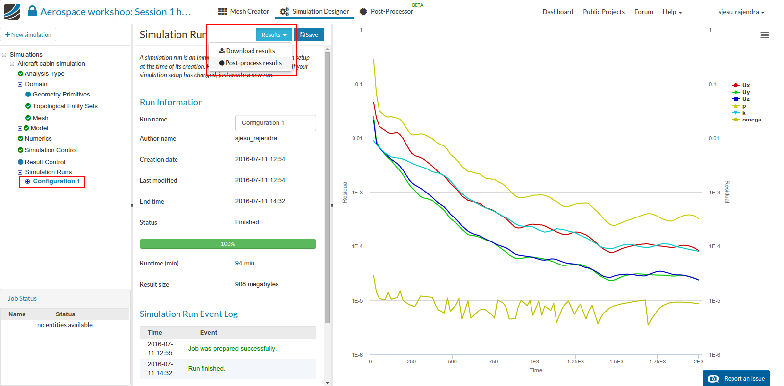
- The simulation takes between 90 to 100 mins to finish.
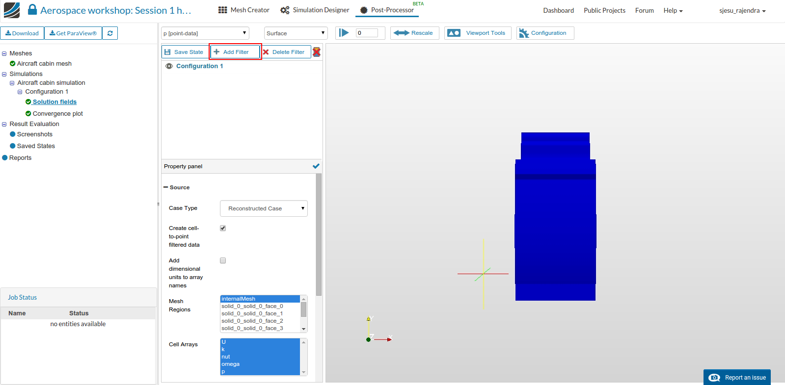
Post-processing
- Once the simulation is over switch to obtain the results by clicking on Post-process results under Results.
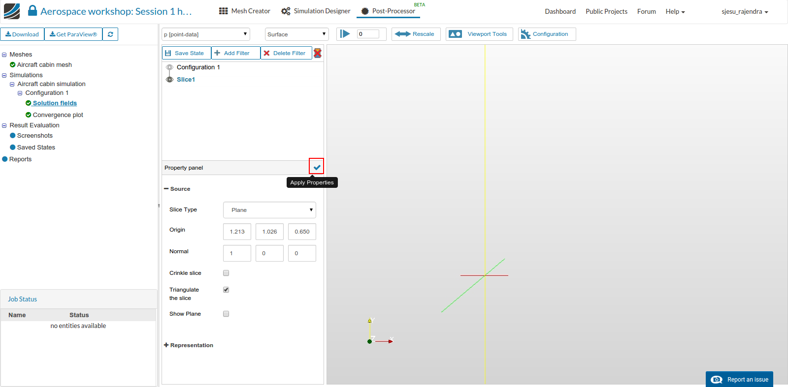
Slice Filter (2D):
- Select the solution field (‘Configuration 1’ in our case) and click Add filter option and select Slice.
-
Apply the following slice properties and click the ‘Tick’ icon to apply.
Slice type - Plane
Origin - default values (1.213, 1.026, 0.650)
Normal - (1, 0, 0) -
Then Rotate in the viewer to visualize the slice.
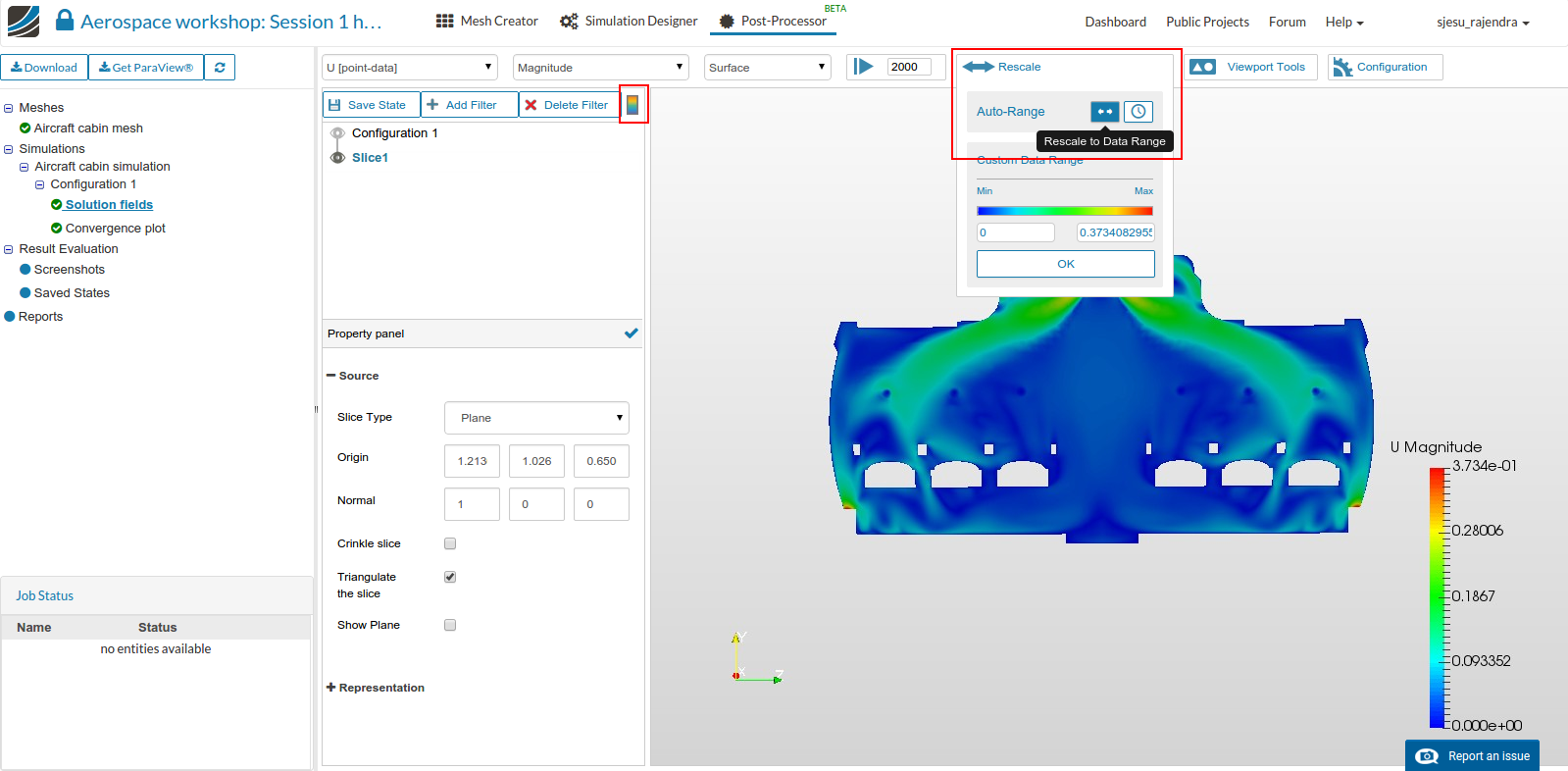
- Select the velocity data U [point data] - go to the last step as shown below.

- Click on the ‘Color bar’ below the selection panel to view the ‘legend’ bar and re-scale it to data range.
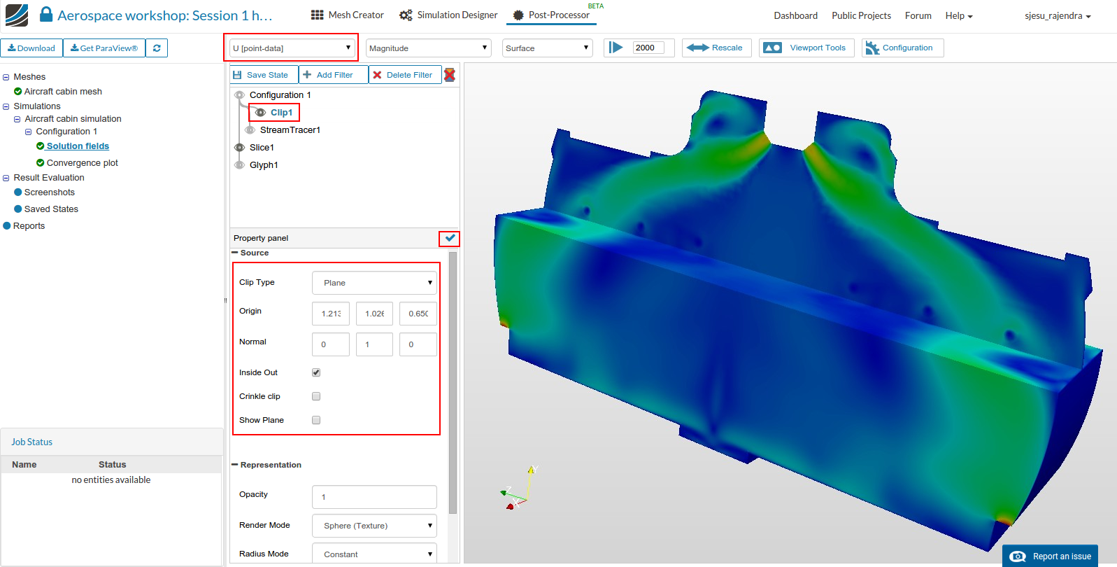
Clip Filter:
- A clip of the domain (3D) can be obtained by clicking on Add filter and selecting Clip option. Enter the following values and click the ‘Tick’ icon to apply.
Clip type - Plane
Origin - default values (1.213, 1.026, 0.650)
Normal - (0, 1, 0)
Streamlines:
-
Click on the solution field (Configuration 1), Add filter and then select Stream tracer in order to get the flow streamlines. Change the display field to U [point data] and enter the following values to create a line source stream tracer (Please leave the other properties with default values).
Vectors - U
Maximum Streamline Length - 10
Seed Type - High Resolution Line Source
Point1 - (1.225, 1.75, -0.2)
Point2 - (1.225, 1.75, 1.5)
Resolution - 100 -
and click the ‘Tick’ icon to apply.

Velocity Vectors:
-
Glyphs can be added to get an overview of how the velocity vectors look like. This can be done by clicking on Add filter and selecting Glyph. Enter the following property values.
Glyph type - Arrow
Scalars - None
Vectors - U
Scale factor - 0.15 -
and click the ‘Tick’ icon to apply.

- Similarly perform the post-processing of the configurations and compare!


