It is my understanding that e1 and e3 are coordinate vectors for anisotropic porous media. So if your media is isotropic you’ll just use (1 0 0) and (0 0 1) respectively.
as @dheiny mentioned, we are working on a fan BC that addresses
and
We expect to bring in to the platform in 2-4 weeks. The first version supports uploading a fan curve CSV file. An analytical function support will be added later.
Regarding the porous media questions,
- Unit vectors e1, e2, and e3 define the porosity coordinate system and correspond to porosity coefficients \alpha=(\alpha_1, \alpha_2, \alpha_3) and \beta=(\beta_1, \beta_2, \beta_3). This means \alpha_1 and \beta_1 are in the direction of e1 and so forth. Same applies to the Darcy-Forchheimer model.
- \rho_{ref} is the reference density. In compressible simulations it must be provided to calculate source terms.
And the two examples:
- 1D flow resistance, let’s say along e1, would mean \alpha = (\alpha_1, 0, 0) and \beta=(\beta_1, 0, 0). To comply with your notation, we’ll have k_1=-\alpha_1*\rho_{ref} and k_2=-\beta_1*\rho_{ref}. Now you only need to provide the face normal as e1.
- To have an isotropic medium, porosity coefficients should be the same in all directions, i.e. \alpha_1=\alpha_2=\alpha_3. Sames should apply to \beta. The rest is similar to the first example.
The reason porous media is not available for incompressible simulations is mainly historical. We will add it in near future.
Babak
1 Like
Hi,
I am starting to setup a test case (just a tube with a end porous zone).
Looking for examples in the library i found the “gas flow through catalytic converter”.
Here de porous zone is defined with some parameters:
Darcy-Forchheimer type
d = (10000, 10000, 10000)
f = (1000, 1000, 1000)
e1 = (0.1, 0.7, 0.1)
e3 = (0.7, 0.1, 0.1)
I don´t see any physical sense in the e1-e3 axis definition.
In addition, I would say it does not matter the e1-e3 definition if the d/f parameters have the same x-y-z component. Is my appreciation correct or am I losing something?
With all this, a “loss” source term is defined (S), after spending quite a lot of time checking, the dimensions are: from documentation ----> alfa=[1/s] beta=[1/m]
From my check: -----> S= [kg]/[m3] * [m]/[s2] = [Pa] / [m]. ¿right?
Now the configuration shall be assigned to a volume region.
I want to match a given pressure loos = f(speed) curve. i.e. from a filter datasheet.
Volume region shall be defined as filter approx. size (i.e. a thin hexaedral)
How can I convert to alfa-beta parameters to match the filter curve pressure loss?
I could use:
region with flow-wise dimension = L1 (in “loss” direction)
alfa-beta set so S term gives (S * L1) = a certain amount of [Pa], depending on speed.
Please give some feedback I am a little loss there…
Regards
I have been trying a really simple test case with the following parameters:
- incompressible turbulent k-e, steady state
- 200m diameter tube
- 1m length + 100mm porous zone + 1m lenght, length aligned with z axis.
- Auto Snappy Hex for internal flow meshing. Quality OK.
- BC: Vz=3m/s inlet, pressure 101300Pa outlet.
- Fixed coef. porous medium: alfa=0,0,0 beta=1e6,1e6,1
- e1=(1,0,0), e3=(0,0,1) aligned with main axis
- numeric schemes from library example (catalityc converter)
Results:
Run1) very inestable residuals with low relaxing factors (0.2 pressure, 0,4 rest, smooth solver for pressure).
Run2) very inestable residuals with VERY low relaxing factors (0.1 all, smooth solver for pressure).
Run4) improvement with isotropic medium (b=1,1,1) both with very low relaxing factors (0.1) and low relaxing factors (0.1 pressure, 0,3 rest) (Run5), BUT no convergence
this is quite discuoraging 
Hello,
Indeed, following the description of @gholami if we have all the parameters for d and f are the same, we will deal with isotropic porous medium and the choice of coordinate system will not have an influence.
Correct.
For the behavior of the porous region and the calculation of the coefficients based on the properties of the material (diameter and porosity), please refer to page 34 of the following document by Di Stefano
Please share the project with the community so we can take a look at the configuration in detail (a public link would be best). We are dealing with advanced models and even though the geometry is simple, many factors might influence stability (most of the time it is the geometrical setup and boundary condition choice and placement). Without seeing the case it is virtually impossible to say what parameter will make it work.
Looking forward to seeing the case.
Best,
Pawel
Hi @jpola,
yes, porous media modeling in simulation can become quite tricky sometimes as the method itself is quite complex. I’ll check your setup and see what hints I can give. Also @Milad_Mafi, having experience with porous media, could you take a look as well?
Thanks,
David
Hi @jpola,
I have taken a brief look at your project and also done a number of sample runs to see what could be the issue.
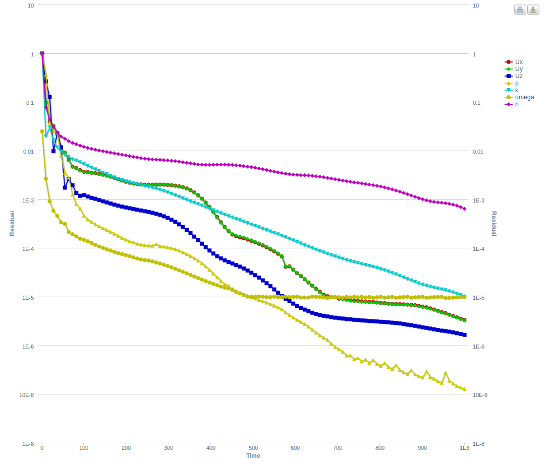
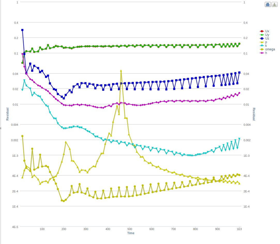
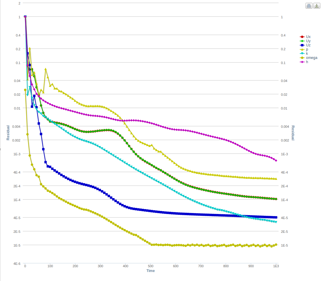
So, I have done 4 case studies of analysis type “Compressible , Turbulent (K-OmegaSST) , Steady State with Porous Media” with your geometry .
For these cases the following were kept exactly the same;
1- Mesh
2- Model
3- Initial Condition
4- Boundary Conditions
5- Numerics and simulation control
So the only thing different for the cases was the “Porous Media settings”. Below are the details and the convergence plots.
Case-1 : with the 'default values of Darcy-Forchheimer Coefficients ’
Case-2 : with the ’ Fixed Coefficients using your values’
Case-3 : with the ’ Fixed Coefficients, but using lower order values compared to your values’
Case-4 : with the ’ Fixed Coefficients, but using default values’
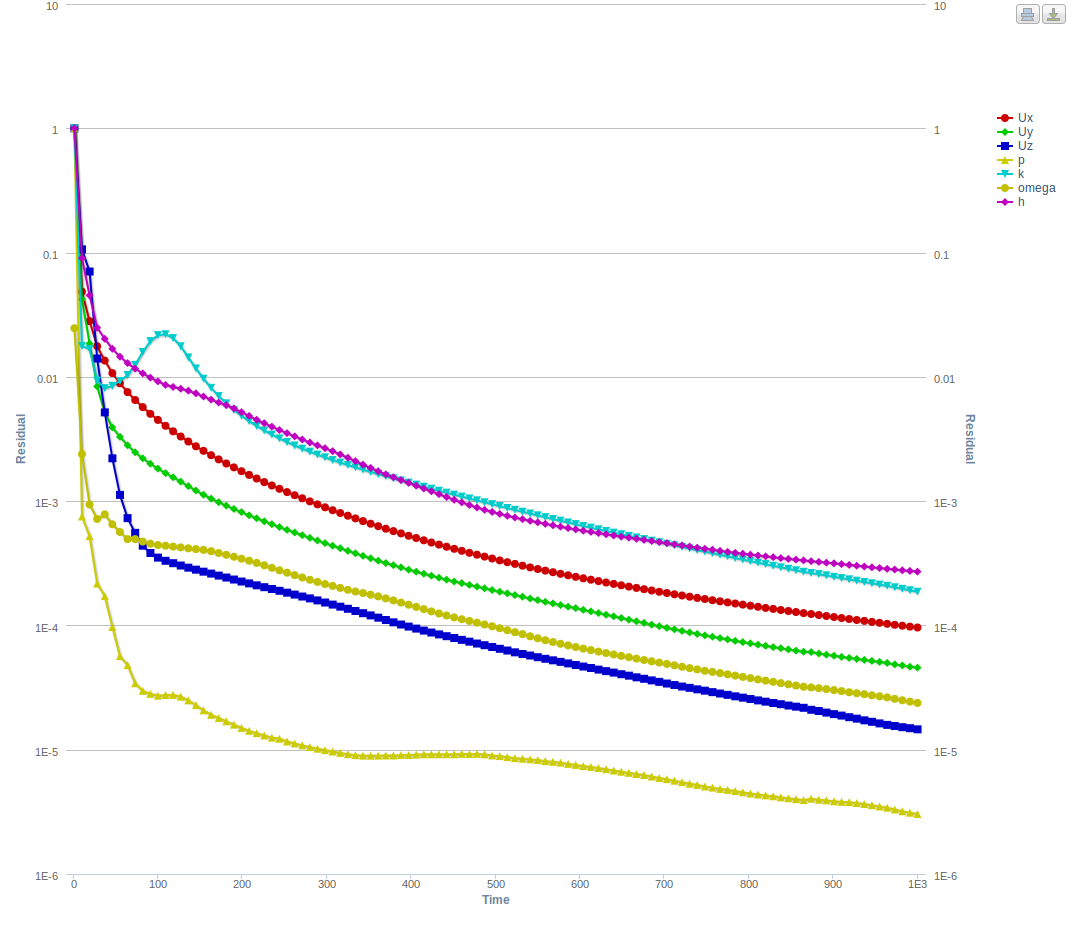
Firstly, based on these plots I see good convergence for Cases 1, 3 and 4 in comparison to your case. Especially when comparing case 2 and case 3, where the only difference is the order of the values.
Secondly, based on the results (not shown here for simplicity) I observe a pressure drop across the porous region for Cases 1, 3 and 4 , that should be expected. While, Case-2 there seems to give a pressure rise. Now I’m not sure if that is what you would expect but it could be a reason for the oscillating behaviour of the residuals.
If you do expect a ‘pressure rise’ for the selected coefficients ( and are sure about the values) then another reason for an oscillating residual behaviour could be a course mesh. Perhaps you could try with a fine mesh and still if you get an oscillating behaviour then it would perhaps mean that the flow is undergoing transient effects with these values of Porous media and can not reach a steady state, so no relative convergence exists for a steady state analysis. Thus you would require a Transient analysis to get to a more relative converged state.
Lastly, It is generally recommended to use low relaxation factors in the numerics for such a compressible case to avoid instabilities and divergence in the first few iterations. ( for these cases they were the same)
Thus, as can be observed from the cases, the Porous media Coefficients have a significant effect on the flow topology and in getting a converged result.
I will send you the link of the Project with these cases in a private message soon.
I hope these observations will be helpful for you and if I have missed something then please feel free to let me know.
Best,
Ali.
1 Like
Thanks Alí,
I intend to use the region as a black box simplification of a passive element with a delta_P=f(speed) curve. I.e. some grille or filter.
So it should cause a pressure drop increasing with speed.
From platform documentation doc the source term is negative with positive coeficients. So with alfa-beta positive the term is negative.
It happens the same with Darcy-Forch. source term. So if your mu-f terms are also positive, no idea why appears that behaviour about rise in pressure, it just doesn´t make sense.
I would like also to clarify how prorus region dimension (i.e. length) affects to total pressure loss source term [Pa]/[m], please somebody give an example with some alfa-beta, speed and dimensions.
Regards
Hi @Ali_Arafat ,
In case 3 (my porous region values, but lowered) as far I could check you just have reduced the beta x-y factors from 1e6 to 1000.
My objective was to assure that the flow resistance is 1D in z axis, and very high in x-y, is that a cause of inestability? is it recommended to limit the difference to 3 orders of magnitude or so?
This is an example of a filter curve I want to simulate: If I set the depth of the zone as the filter approximate depth size, how the alfa-beta factors shall be related to the curve and depth?
filter curve
Regards
Hi, @jpola
For Case 3 your original values were reduced 2 orders down, so beta x-y factors from 1e6 to “10,000”. This was just to check how the magnitude effects the convergence and results. So clearly it has a significant effect.
I would say the values you are using are related in a way to the instability, so you have to be sure if they are correct with respect to the required inputs and the way its implemented. I’m not sure if there is any limit of 3 orders, as the lowered values I took were just for test purposes and not based on any recommendation.
Regarding the formulation of the coefficients please go through this short documentation (if you have not already): SimScale Documentation | Online Simulation Software | SimScale
For how to relate alfa-beta to the curve, Babak @gholami will get back to you soon with some description.
Best,
Ali.
First of all, your dimensional analysis is correct: the source term essentially represents a pressure gradient.
Regarding calculation of model parameters from pressure loss curve, with the information you’ve provided, you cannot do this. Here is why (for simplicity I’ll write everything in one dimension):
Let’s assume pressure loss to be a function of velocity $$\Delta p = f(u),$$ which says pressure difference before and after the medium is f(u). However, the porous model $$\frac{dp}{dx} = g(u)$$ represents a pressure gradient inside the medium. If you integrate it along the medium, you’ll have $$\int g(u) dx = f(u),$$ which is of little use since calculation of the left hand side requires knowing velocity gradient across the medium.
Porous model parameters are properties of medium and not the field. For example, you’ll see that in the reference @psosnowski provided, model parameters could be calculated by knowing physical properties of the medium, i.e. porosity and diameter.
Let me know if you would like to discuss this further.
Hi Babak @gholami, sorry abour not using the nice Latex style notation, I do not control it…
Trying to buid on your 1D explanation I would say:
-
For fixed coef. sourcer term I would set :
ro_ref=1, alfa=0 and beta so g(u) = dp/dx = b *u^2 -
u=u(x) in this 1D problem, as assumption I could use a constant linear velocity for a blackbox filter model, i.e. u(x) = u(x0) = u0
-
integrating 1D along x:
integr( g(u) dx ) = integr(b * u0^2 dx) = b * u0^2 * x -
so: delta P = b * u0^2 * L,
L being the “length” of the porous zone and u0 the inlet speed to it.
Now, with a deltaP curve of a filter datasheet, in case I want to model it:
- select length of porous zone L (i.e. depth of real filter bed aligned with flow)
- select beta to match filter datasheet speed-pressure drop curve with:
delta P = b * u0^2 * L,
Alfa-Beta parameters of axis non aligned with “main flow” shall be set high enough to support the 1D assumption (i.e. x3 orders of magnitude, it seems that a very high value can cause stability problems, but no clue why).
A similar setup could be used for linear filter curves using the “alfa” parameter.
Please comment if the previous make sense.
Regards
Your derivation is correct. However, it should be regarded as an approximation. After all, we are fitting two expressions that do not have a direct physical equivalence. In this case, any variations in velocity, due to shape, density change, body forces, etc., violate the constant velocity assumption and result in inaccuracies.
I still think it is a good starting point. As long as L is kept small, external body forces are absent, and thermal variations are negligible, a certain level of accuracy should be maintainable.
Regarding using large coefficients, it is expected to run into stability issues. Large coefficients would mean large source terms in the momentum equation; therefore, you should treat your numerical settings much more carefully. Before doing that though, are you sure you need to explicitly restrict the flow in those directions?
Actually, the motivation to restrict in direction non aligned to flow (i.e. x-y), is just to keep the 1D pressure loss simplification (in z). Think i.e. a straight duct with a thin filter where in z the flow advances and in x-y cannot move due to filter bed.
If a high factor can cause problems, what effect can have isotropic loss factors in this type of application?, if the source term is the same for every direction I suppouse the flow direction shall continue unchanged through the region, and the net behaviour shall be similar to making non flow aligned loss factors higher… If that improves stability and gives same result can be a better option.
Regards
I did some tests simulating a loss factor filter of
(1/2) * K * ro * u^2, with K=280, ro=1,2kg/m3 (air)
With inlet speed 8m/s should give 10752Pa of pressure drop.
Using a “thin” porous region of L=0,01m, this results on
beta=(1e6, 1e6, 16800) alfa=(0, 0, 0) and ro_ref=1 as parameters for the region to match the previous loss factor equation.
Results of simulation including 1+1m or duct before/after pressure drop are:
- region modeled with 2 cells across, v=8m/s
dP=2132, error -80%, not valid - region modeled with 5 cells across, v=8m/s
dP=11166, error 4% - region modeled with 10 cells across, v=8m/s
dP=11489, error 7%
Results with inlet speed 4m/s, dP theoric = 2688:
- region with 5 cells across, v=4m/s
dP=2588, error -4% - region with 10 cells across, v=4m/s
dP=2656, error -1%
Results with isotropic factors beta=(16800, 16800, 16800), v=8m/a:
- region with 5 cells across, v=8m/s
dP=10807, error 1% - region with 10 cells across, v=8m/s
dP=11269, error 5%
My preliminary conclusions:
- previous discussion about how to use the porous region to match a thin filter, perforated plate or similar for pressure loss factor simplifications seems to work
- Number of cells in the region is important, with <5cells the region is not correctly modeled and results are not valid for the example. It is not clear if increasing from 5 cells improves the results.
- For flows non aligned perpendicular to the loss region, a high enough factor shall be used for the non relevant directions, but be aware that a big difference between values causes a lot of stability issues in the solver. I had to test from 3 (as suggested in @Ali_Arafat post) up to even only 1 order of magnitude difference between the factors, to avoid problems of solver stability.
- For flows aligned perpendicular to pressure loss region (as this case), the results using isotropic factors are valid (actually seems better), and are less prone to stability issues in the solver.
Any comment is welcomed
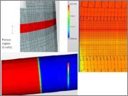
Attached images of the “5 cells across” porous region, L=0,01m.
There is a light difference in the mean speed before and after the region, I don´t know what causes that and if could be a problem,
any comment?
Hello everyone,
I need to simulate a porousZone with an incompressible solver, but I can’t find the option in Advanced Concepts:
Simulation: Incompressible-Steady state-kOmegaSST
Should I enable something else before?
Thanks.
Daniele
Hi @DanieleObiso,
unfortunately porous zones for incompressible flow sims are right now not supported yet - it’s in the works!
Best,
David
Hi @akosior,
yes there’s progress regarding porous media for incompressible but we don’t communicate release dates as we’re working agile in software engineering. So there’s never a 100% guarantee that an anticipated release date will be kept. Will inform you as soon as it’s there.
Best,
David