Tutorial Updated 2018-11
Recording

Introduction
The FEA Master Class: Session 1 covers the categorical procedure for obtaining a solution, independent of the mesh. Since the mesh is refined to the extent that further reducing the fineness does not have a sizable impact on the solution, it is known as Mesh Independence Study. A Mesh Independence Study can be thought of as one of the ‘Best Practices’ in engineering simulation.
During the design phase of a product, engineers deem some solution fields to be decisive factors in the final design. Since the solution fields assume a rather significant role in the conception of a product, they need to be quantified. For this purpose, it is vital to have a solution free of numerical errors.
In this exercise, your task is to utilize the SimScale Platform to setup a local mesh refinement and simulate the resultant stresses on the frame of a bike when a person is standing on its pedals. One of the primary factors in determining the design of the bike frame is to have a factor of safety which is at least two times the maximum stress that the bike would undergo at any point in operation.
To begin with, you have been given the bike frame geometry (bikeFrameFacecuts). Your task is to work with the geometry in order to generate a mesh and refine it in the region near the maximum stresses. Following this, you can setup a simulation and validate it with the provided simulation results.
This assignment is only one part of a Mesh Independence Study. Other aspects of mesh independence include switching to a second order mesh. The curious user may delve deeper into the topic by creating a second order mesh and comparing the results.
Import Project
To start this exercise, please import the project into your workspace by clicking on the link below:
Project Link
Mesh Generation
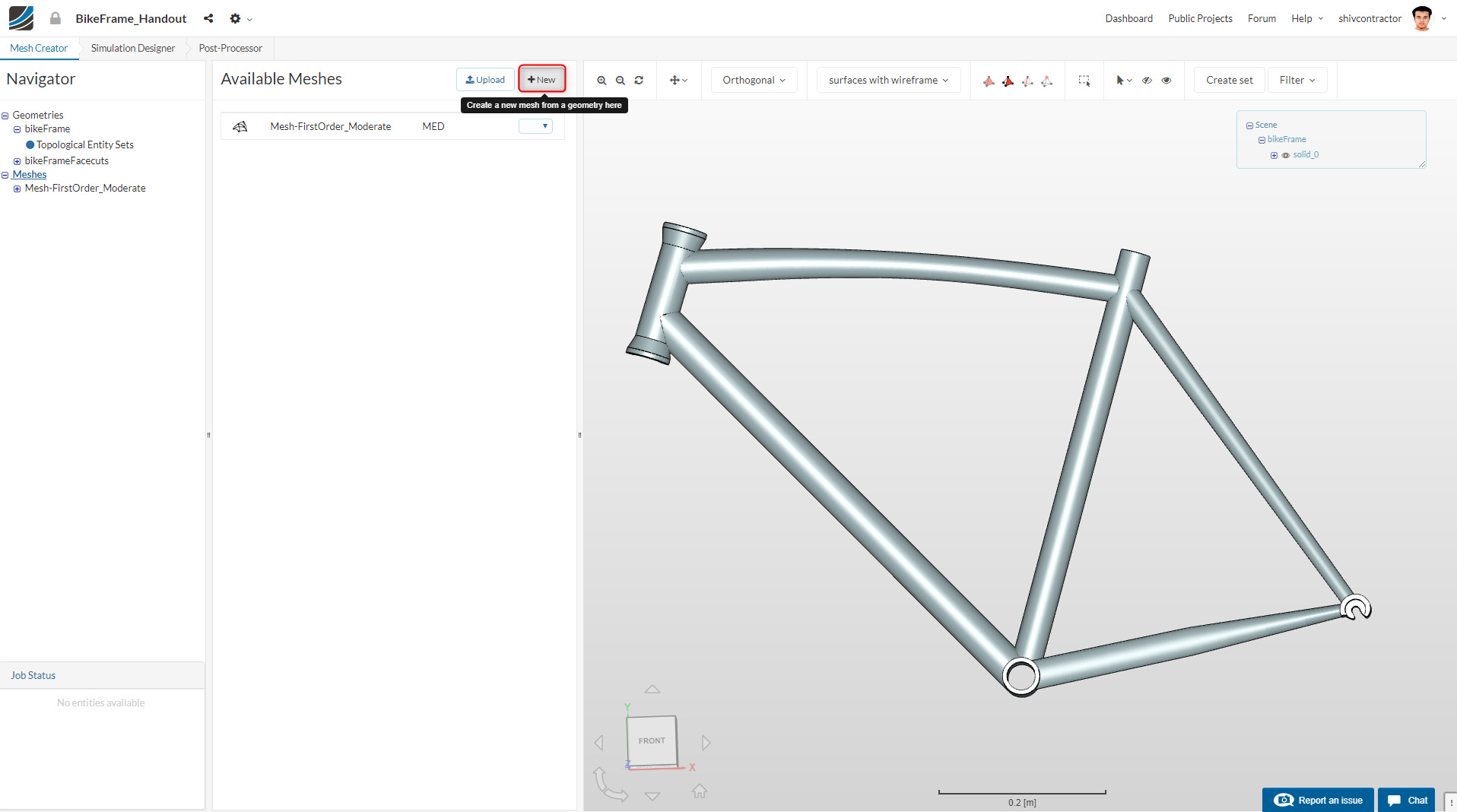
In the SimScale Mesh Creator, select Meshes in the Navigator and click New.
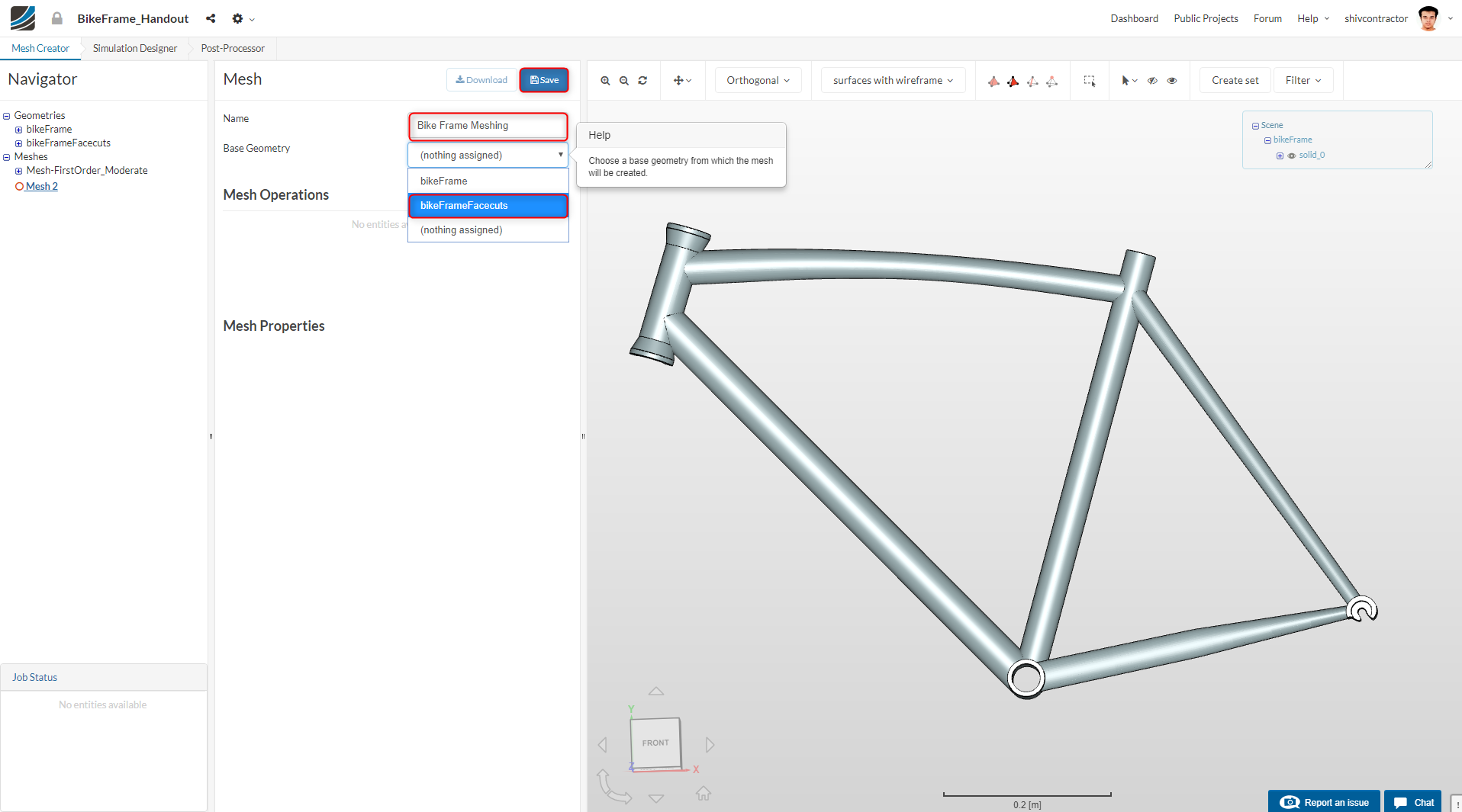
Assign an appropriate Name to your mesh, for example, Bike Frame Meshing, and select the Base Geometry as bikeFrameFacecuts. Click Save.
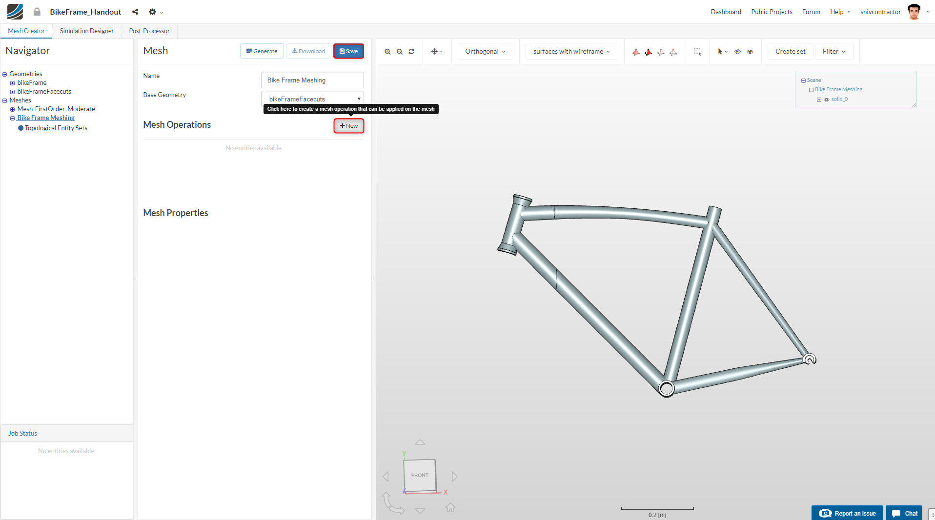
Create a new Operation by clicking on New. A Tet-dominant mesh operation is used for this FEA study.
The global mesh sizing may now be set as follows:
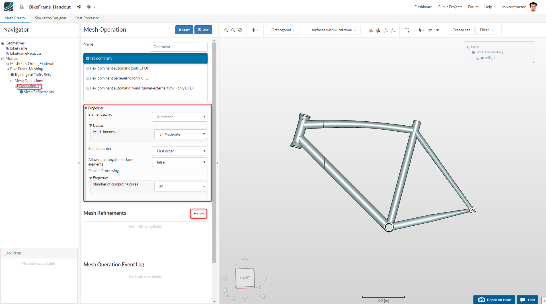
As we already know, this study focuses on local mesh refinements. Proceed to make one by clicking on New.
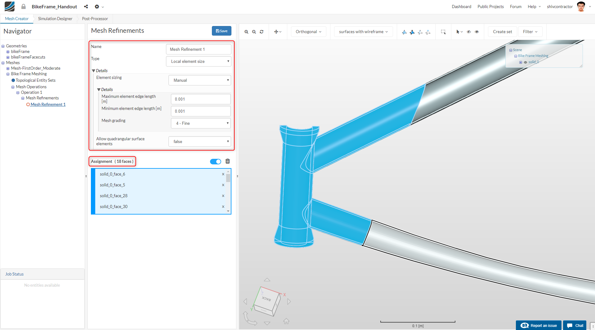
Set the Type as Local element size and the Element sizing as Manual.
Set the Minimum edge lengths and Maximum edge lengths as 0.001 since we want to have at least two elements along the width (2 mm = 0.002) of the bike frame.
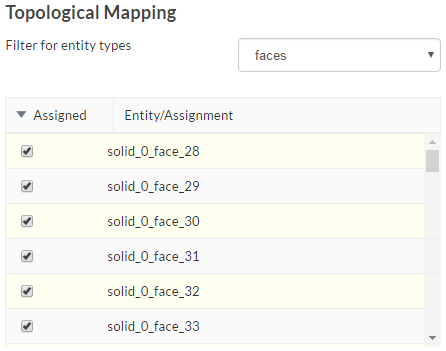
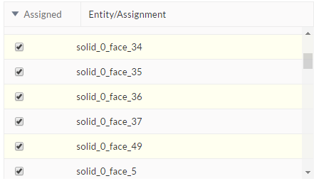
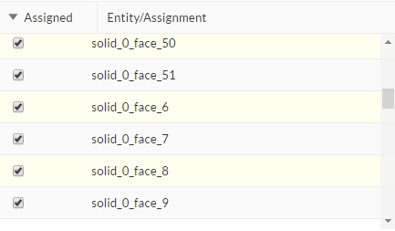
For greater convenience in selection, you can use the Box Assignment Tool displayed on the top right of the viewer. Please make sure that the 18 faces to be refined are selected as shown in the image below:
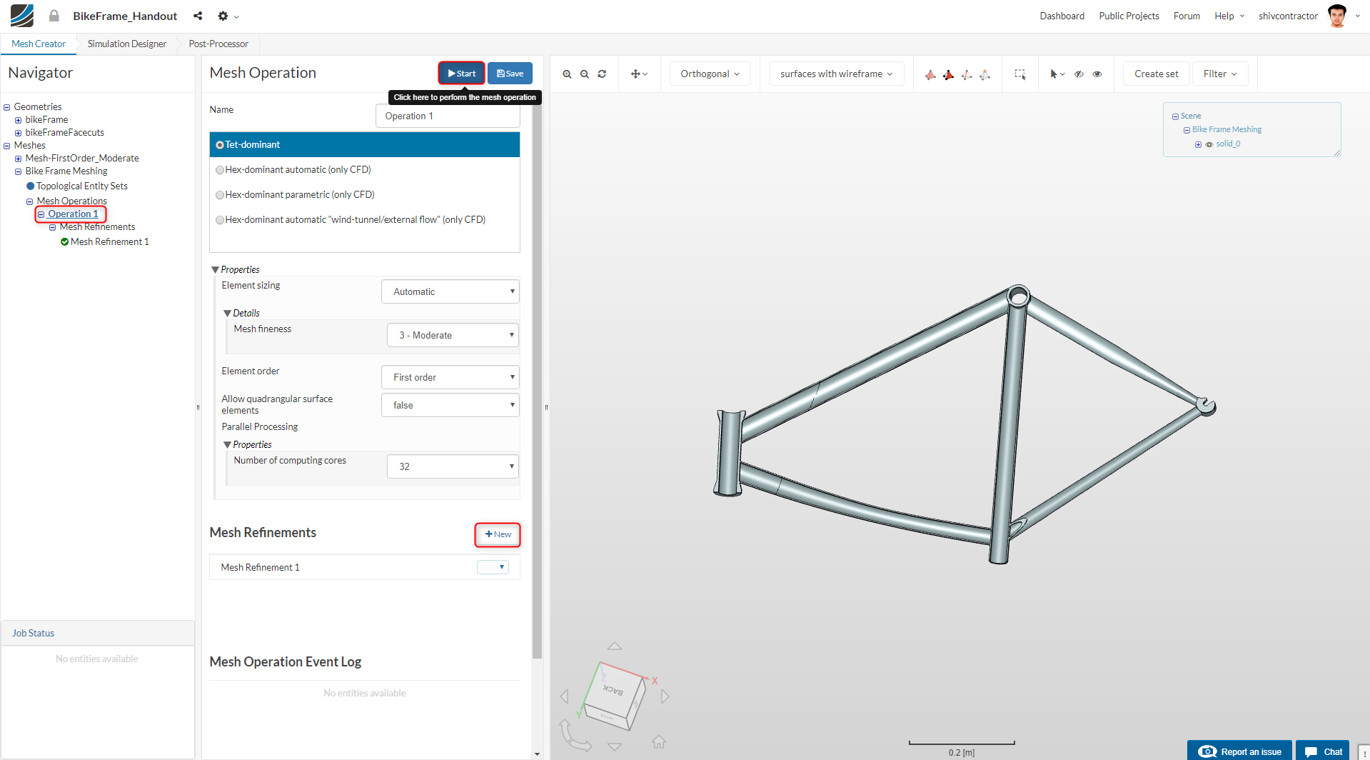
Start the meshing operation from the Operation 1 item in the Navigator
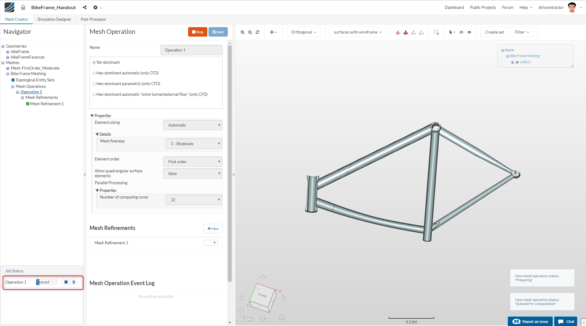
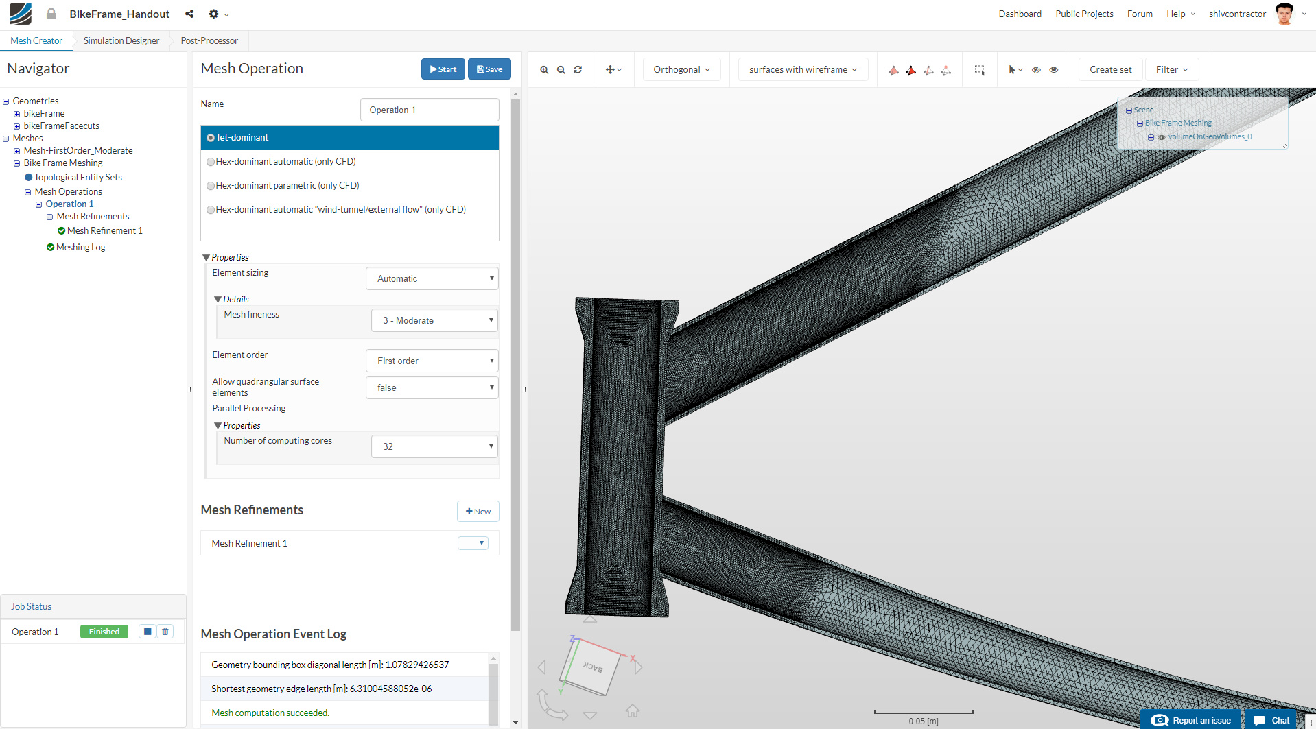
The mesh may now be visualized in the viewer.
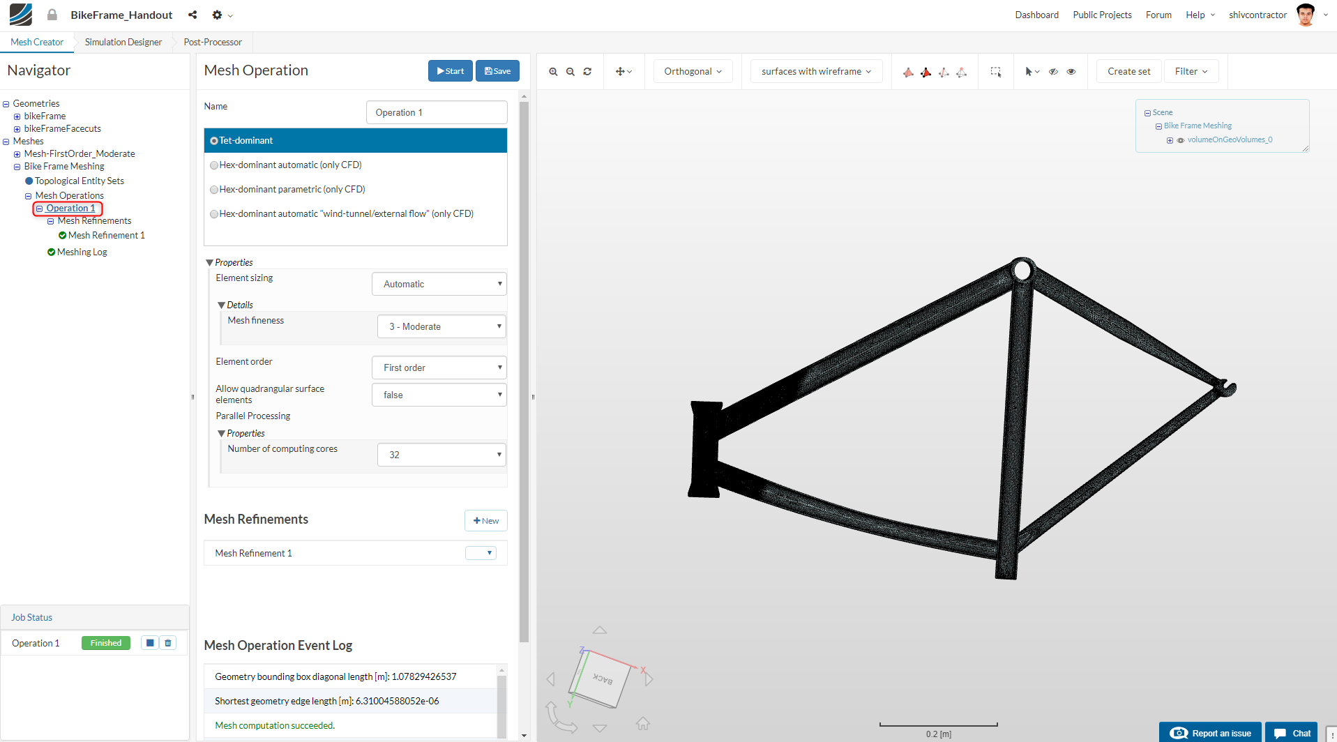
As you can see, the mesh in the selected region is much finer than that of the other components.
Please proceed to the Simulation Setup.
Simulation Setup
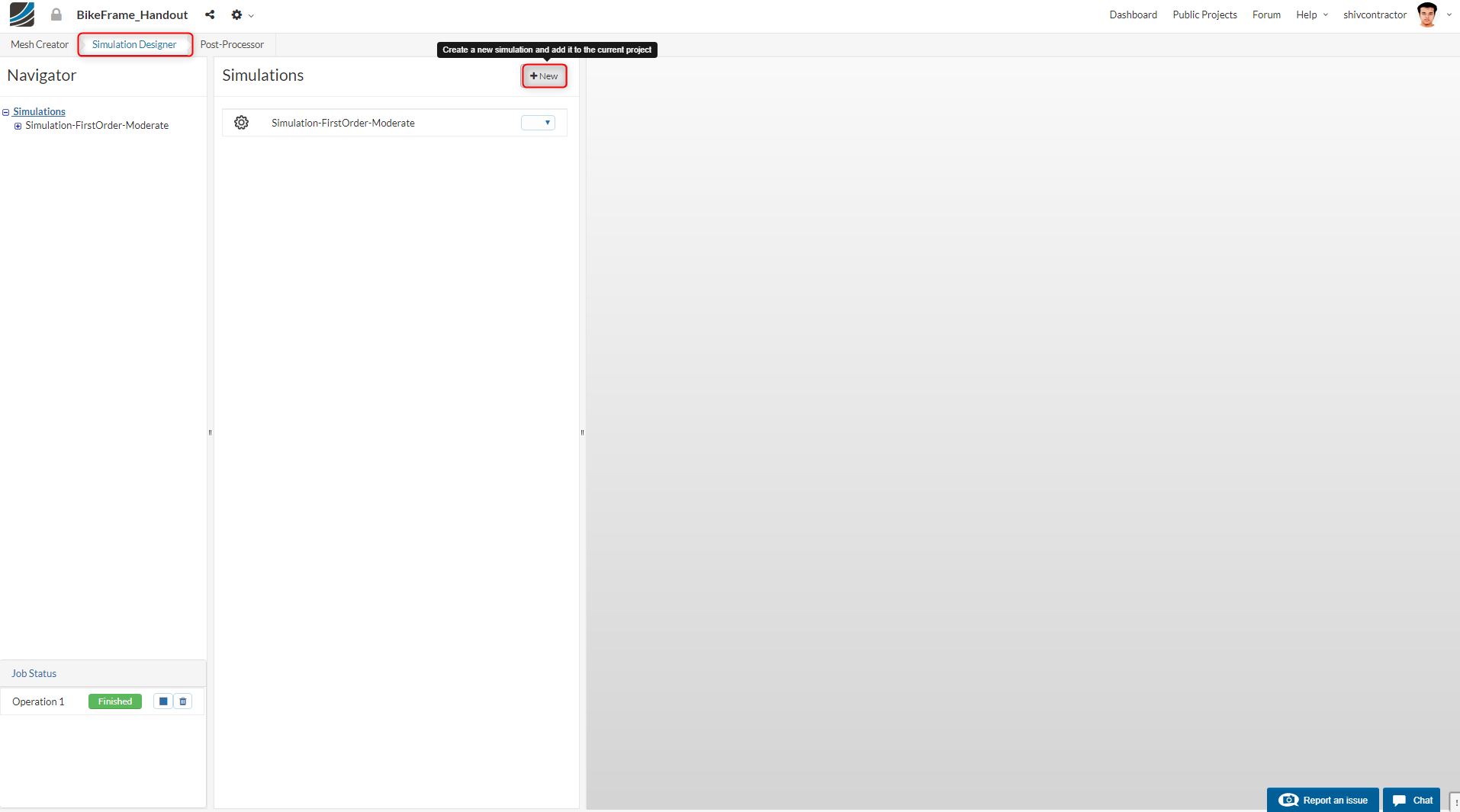
Navigate to the Simulation Designer tab in the SimScale Workbench and click on New to create a new simulation setup.
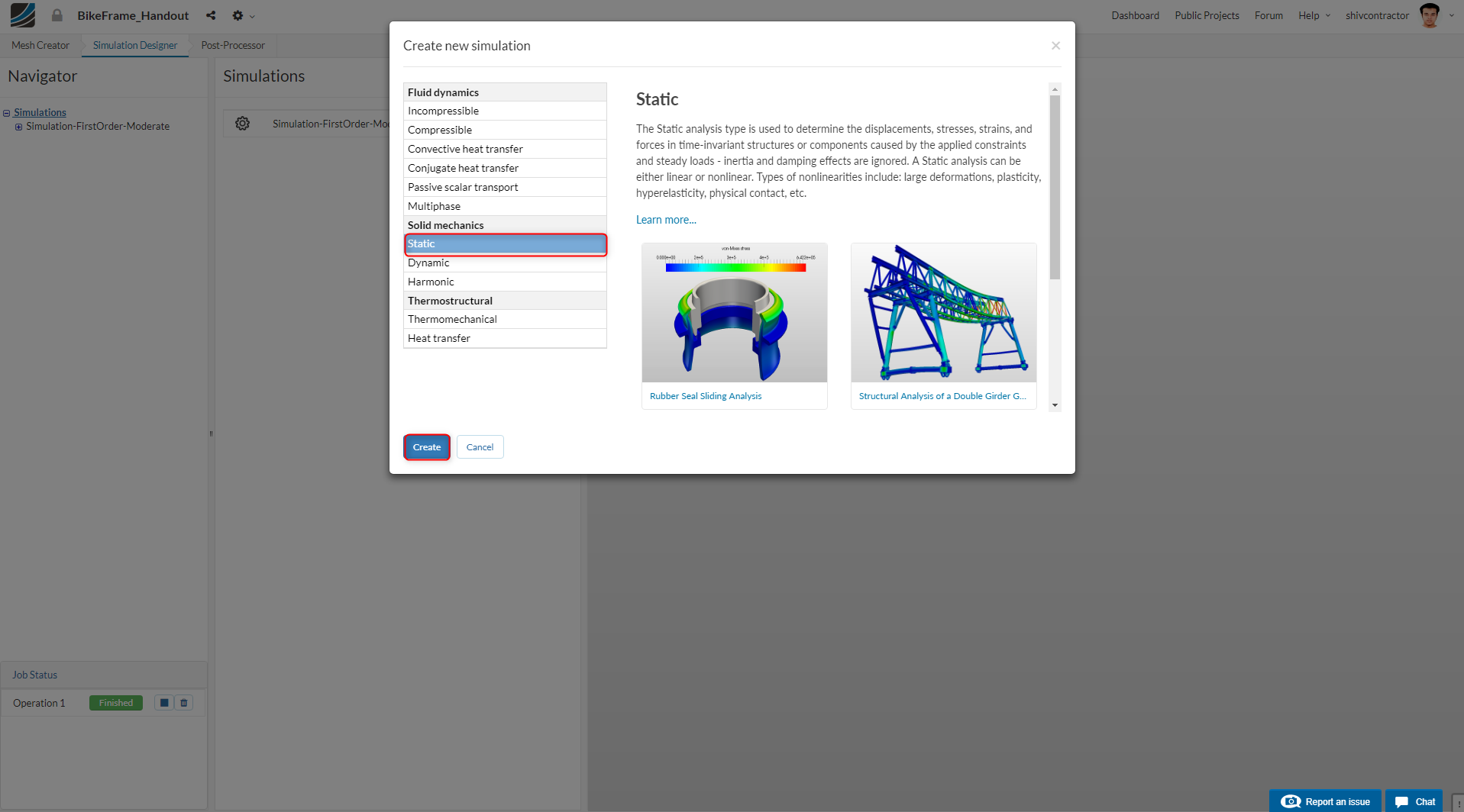
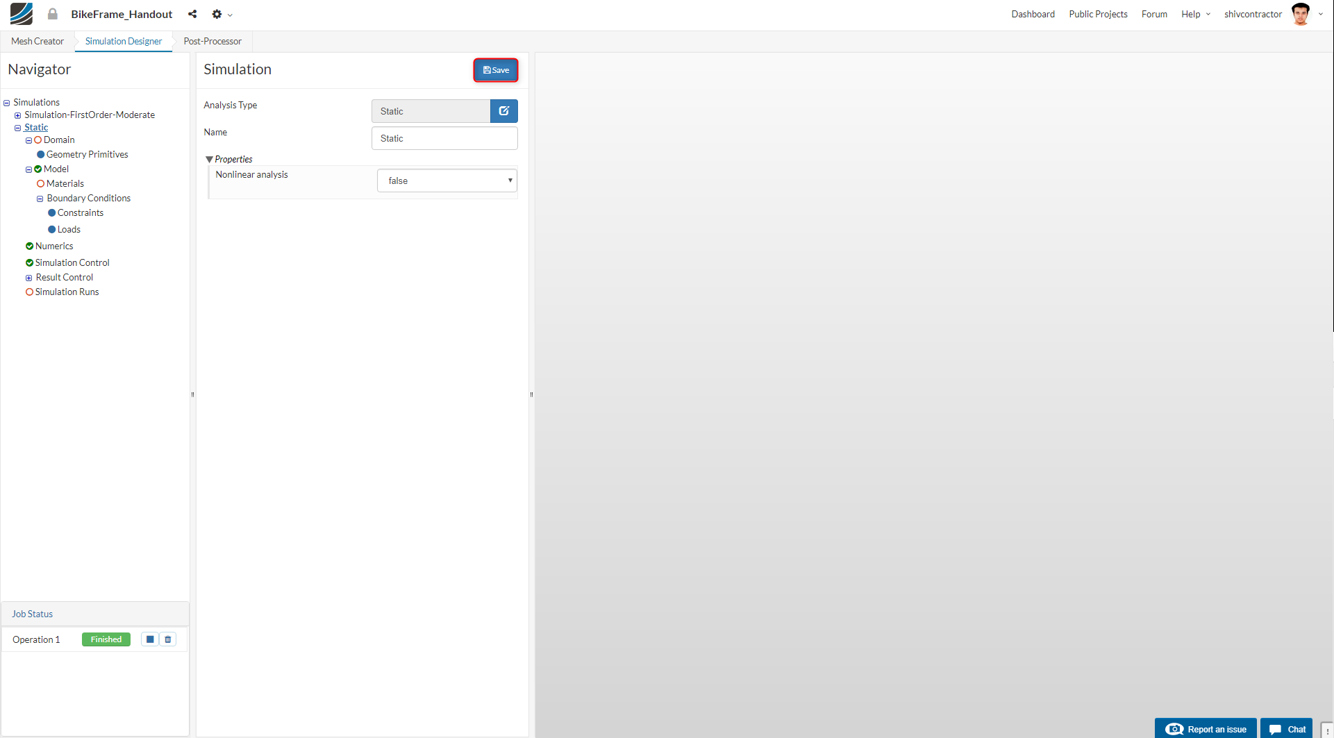
A window will pop up, asking you to select the type of analysis. Click on Static in the category Solid Mechanics. Click Save to close the pop-up.
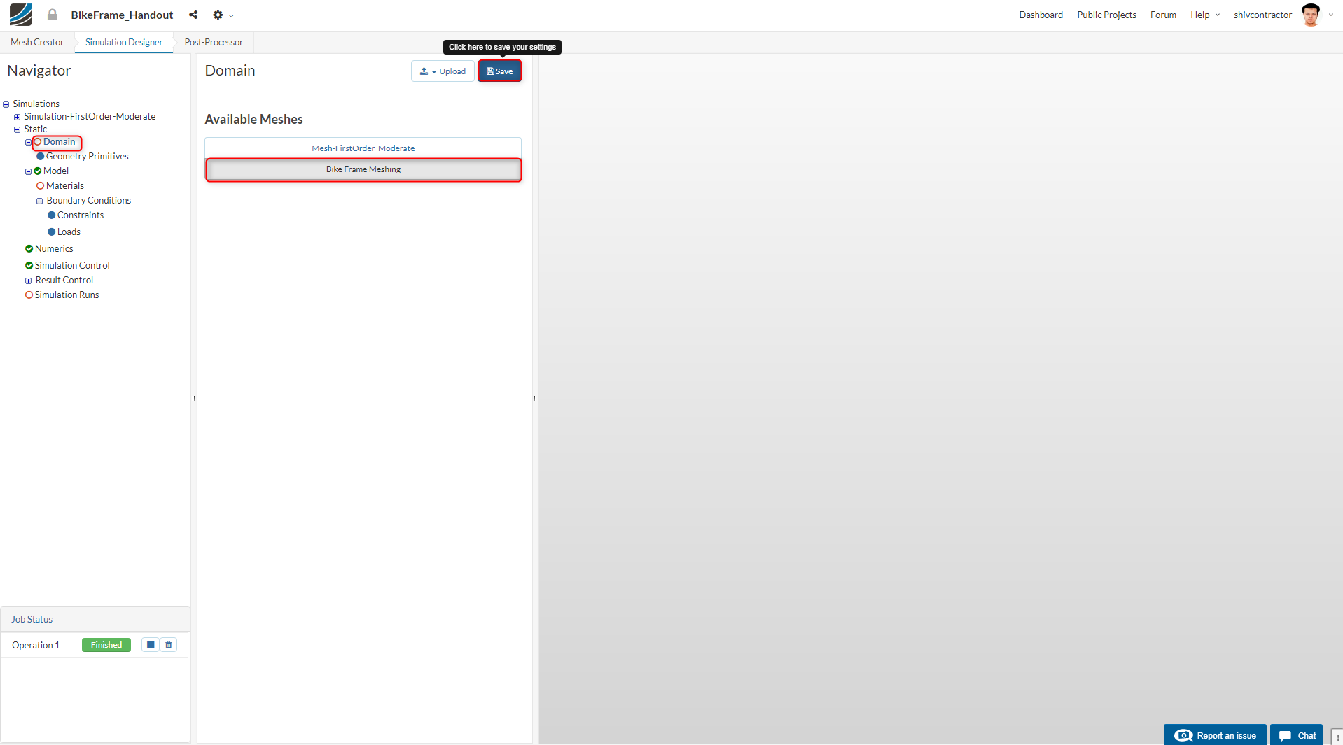
Next, select the mesh that you created, Bike Frame Meshing.
Click Save to store your progress.
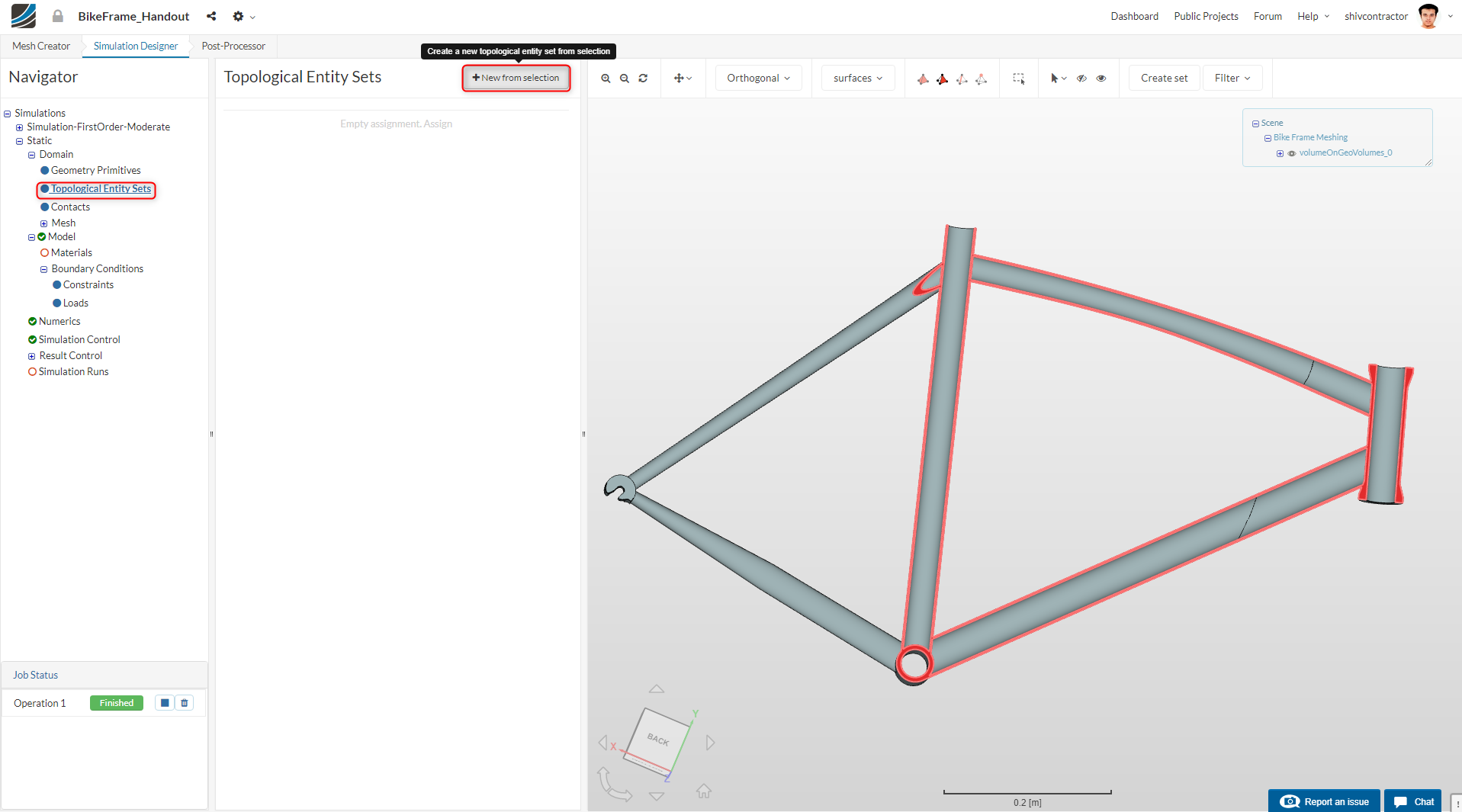
Topological Entity Sets
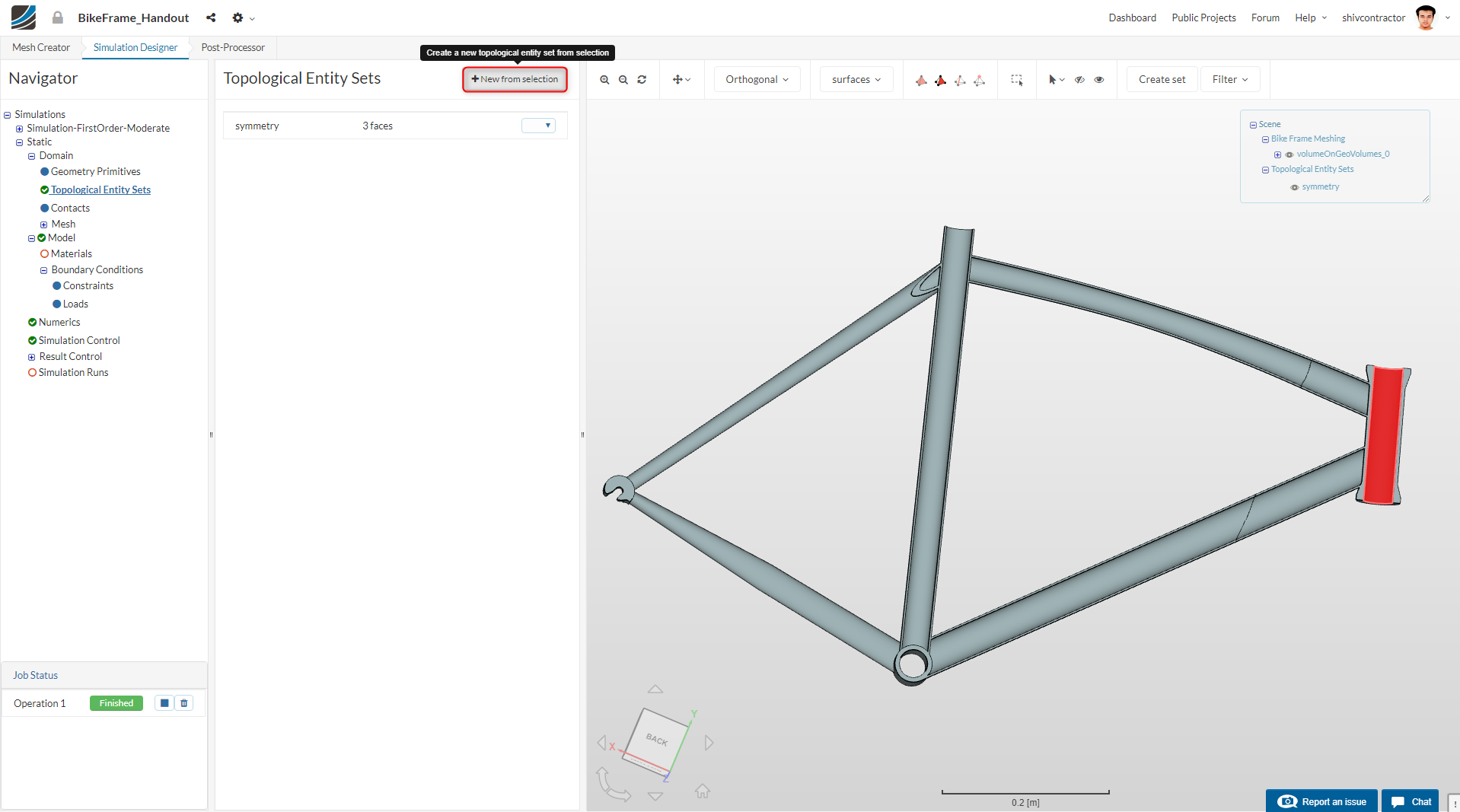
Please create the topological entity sets as shown. Here it is important to note that the topological entities are first to be selected in the viewer, followed by clicking on + New from selection.
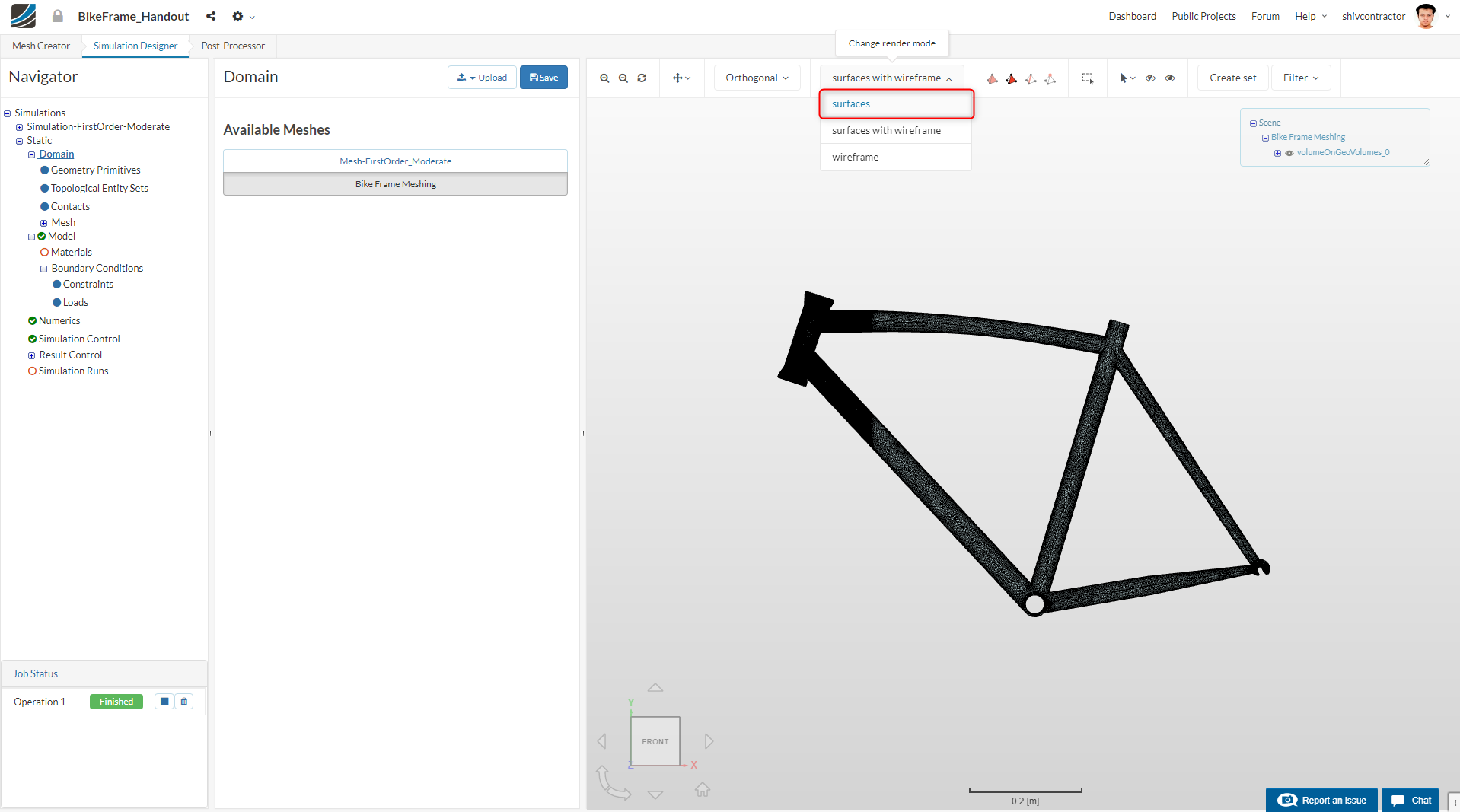
For easier mesh handling, it is recommended to switch to surfaces render mode in the top viewer bar.
Symmetry
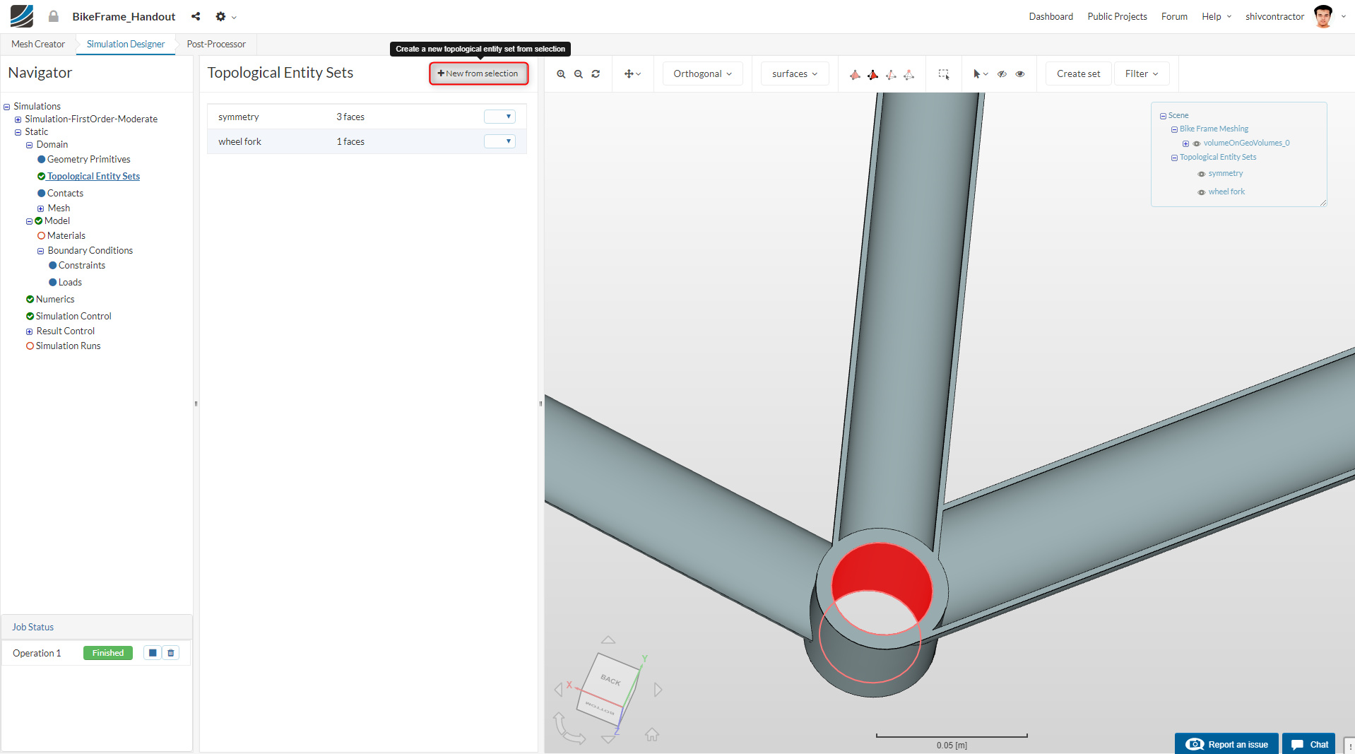
Wheel Fork
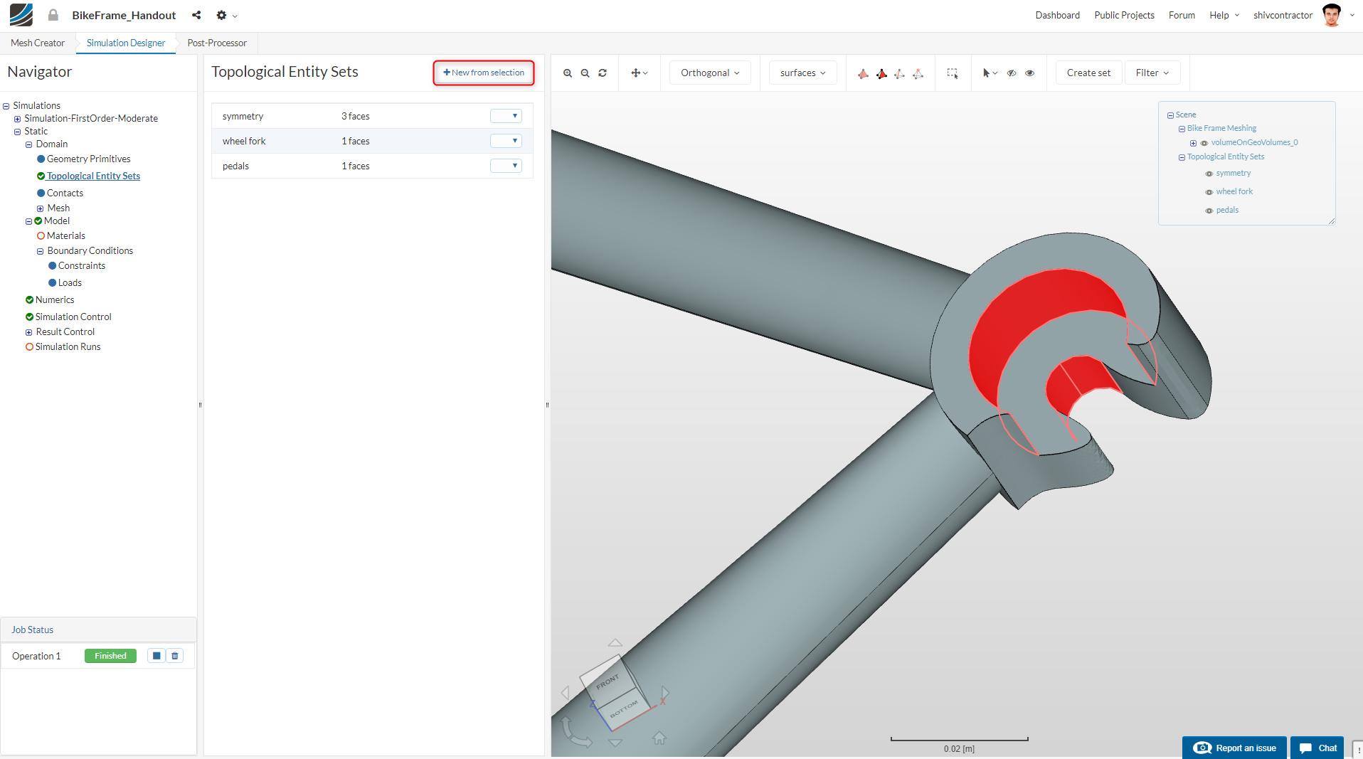
Pedals
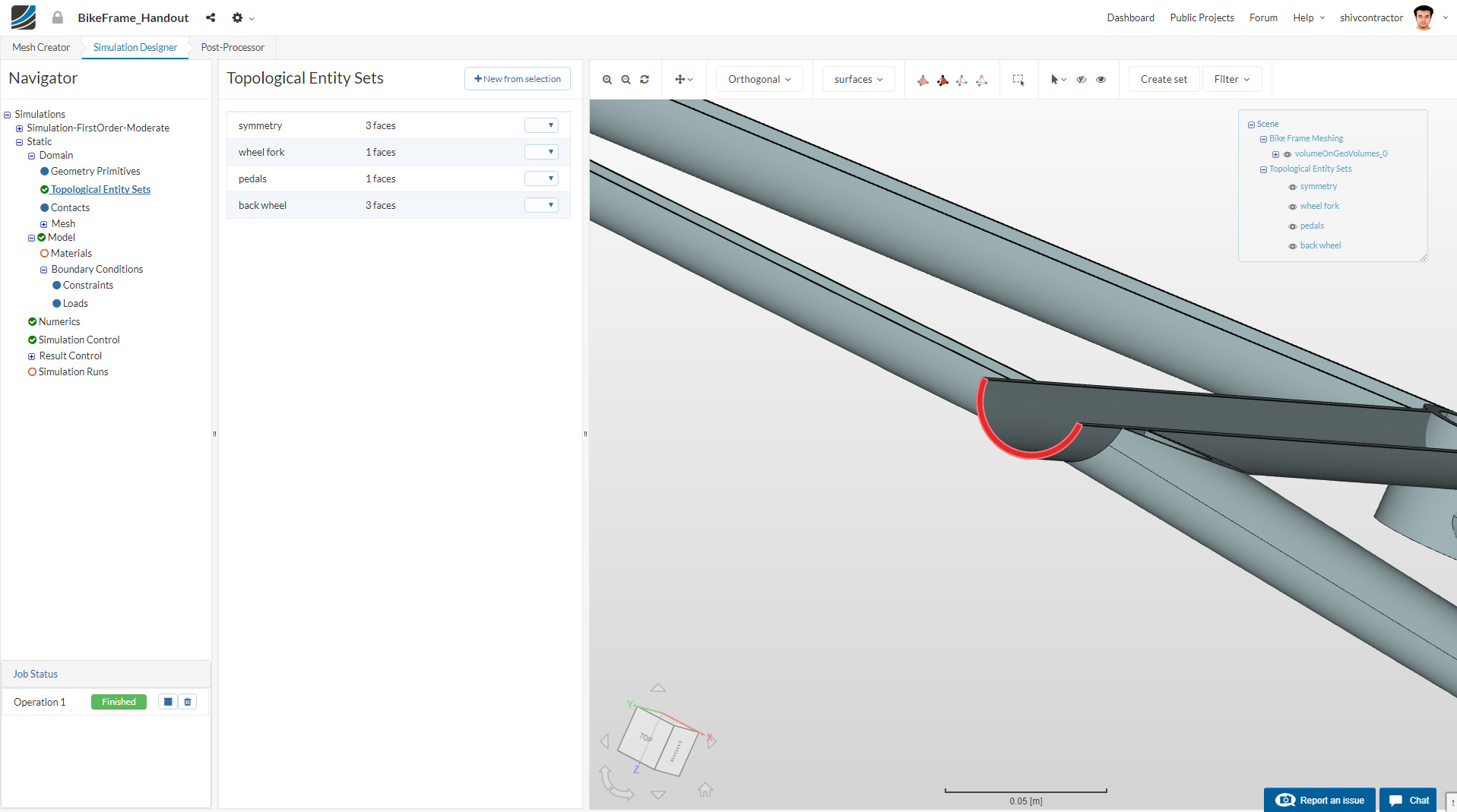
Back Wheel
Seat
On the ongoing task bar, you can see that we have successfully assigned the Topological Entity Sets. We will use these TES to assign Boundary Conditions later in this tutorial.
Material Selection
Please select Materials in the Navigator and click on New.
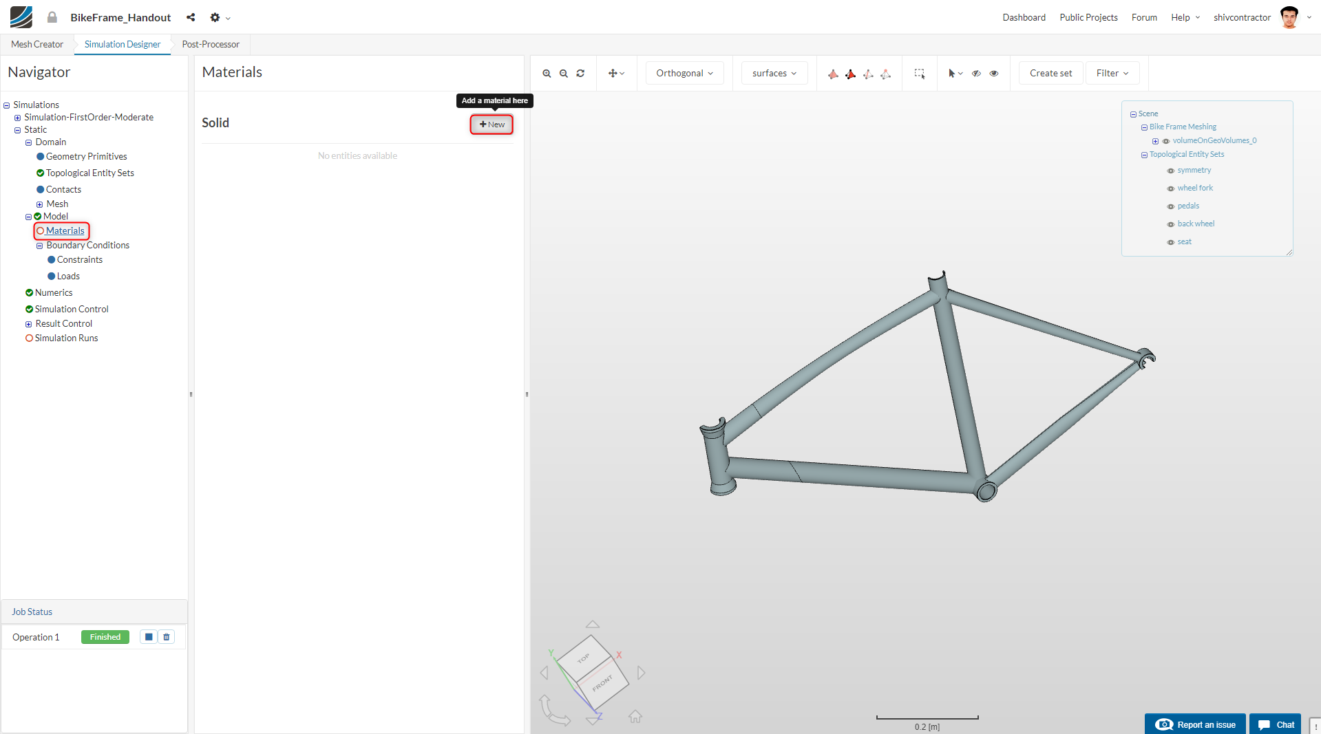
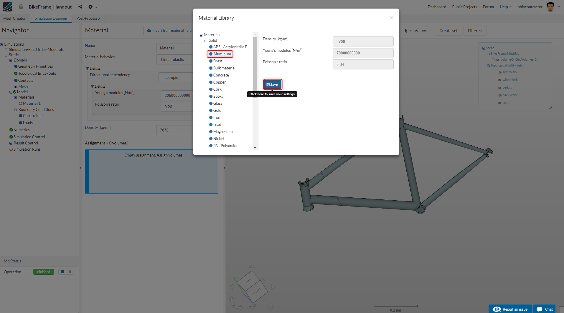
As shown below, make an Import from material library.
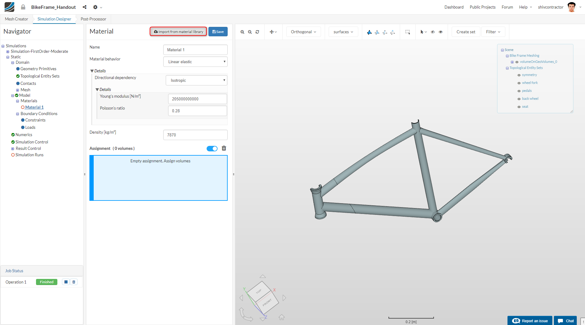
Proceed with Aluminium as the material for the bike frame.
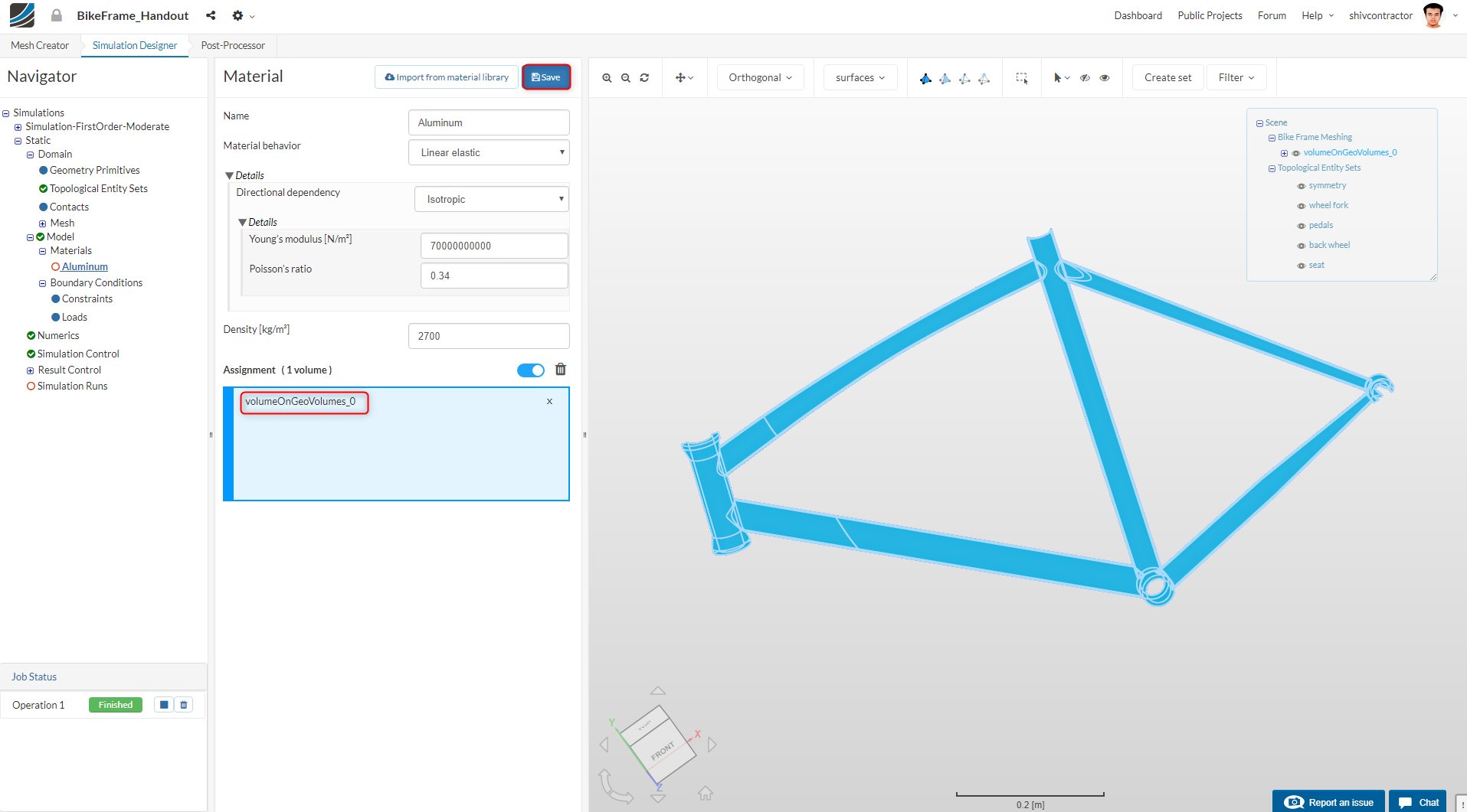
Assign the material to the entire bike frame (volume). To do this, click anywhere on the meshed geometry and highlight the material. Click Save to preserve the material settings.
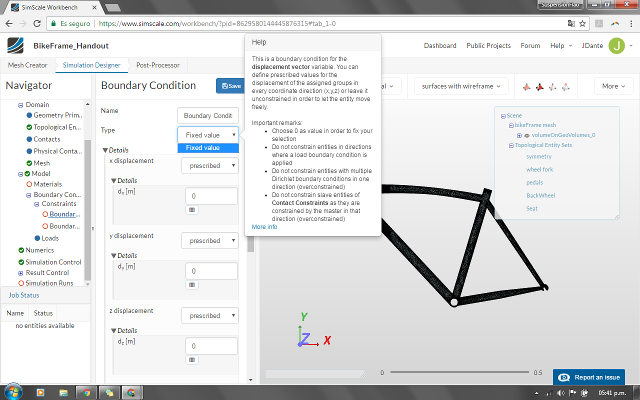
Boundary Conditions
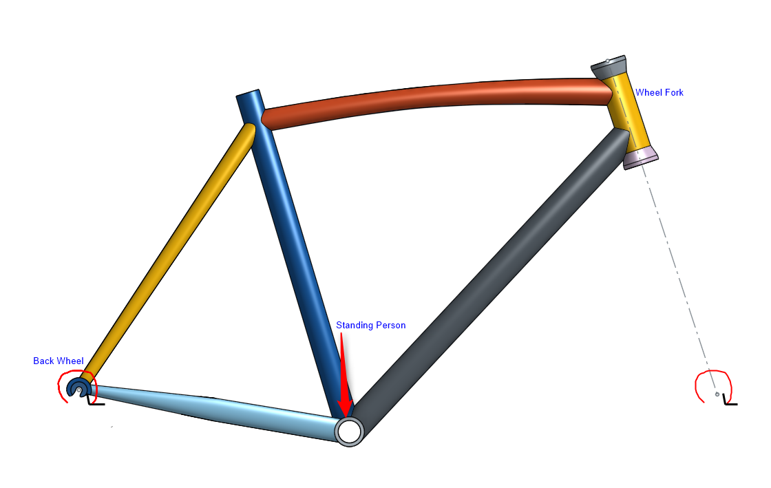
Here is an overview of the constraints and loads on the Bike Frame:
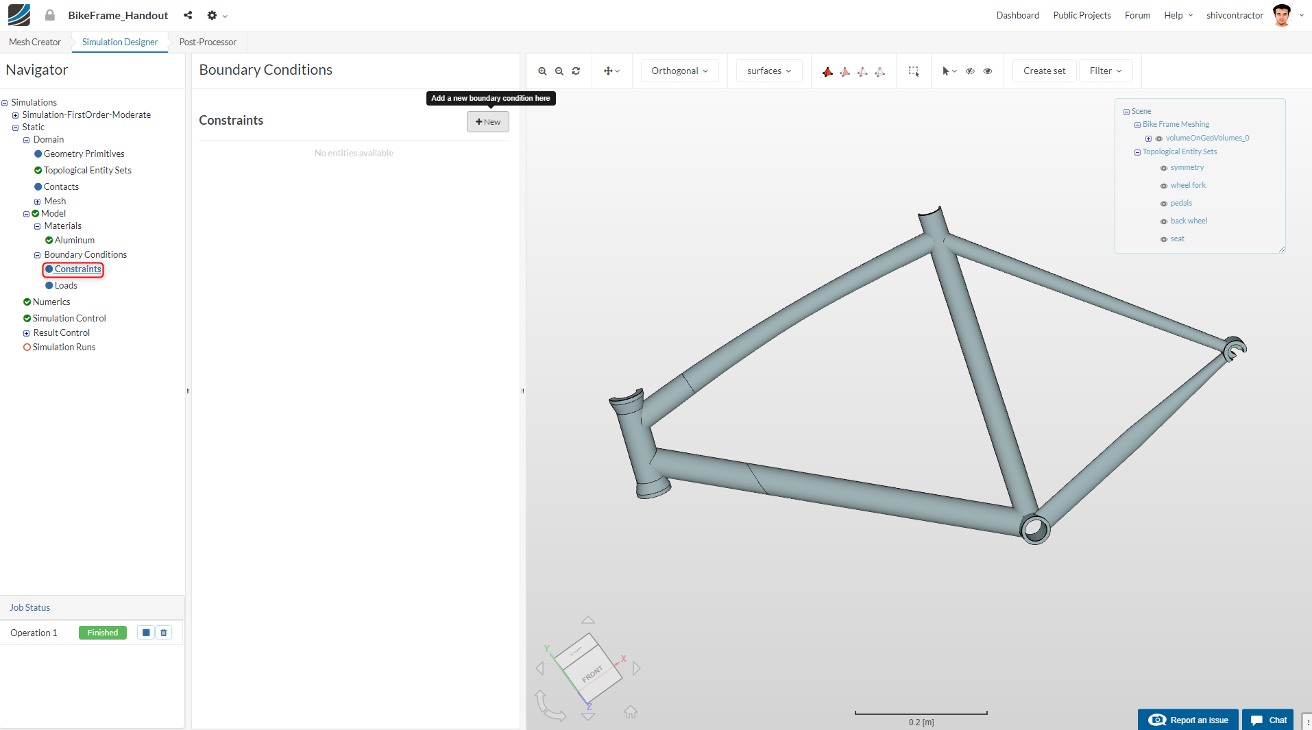
Let us proceed to add constraint boundary conditions. Please click on Constraints and click on New.
The bike wheel is constrained in all degrees of freedom except for the rotation about its axis (Z-axis). Please follow the images below to setup the back wheel.
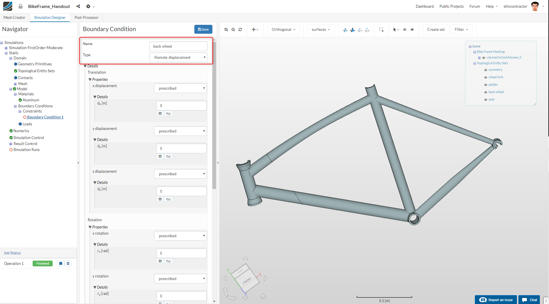
PLease check that the **Deformation behavior ** is set to Deformable.
To add another set of constraints, right click on Constraints in the Navigation bar and select Add Constraints bound
 
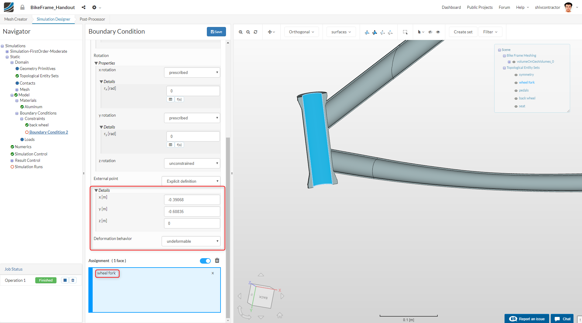
Similarly, the wheel fork is also constrained in all degrees of freedom except two. Give it some thought?
The wheel fork is allowed to translate in the X direction to account for any deformations in the rest of the frame. Also, the wheel fork is allowed to rotate about the mount of the front wheel.
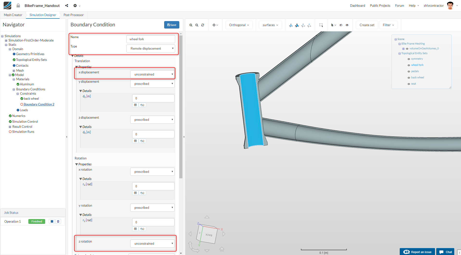
Secondly, the wheel fork is also allowed to rotate about the mount on the of the front wheel. Also leave here the **Deformation behavior ** as Deformable.
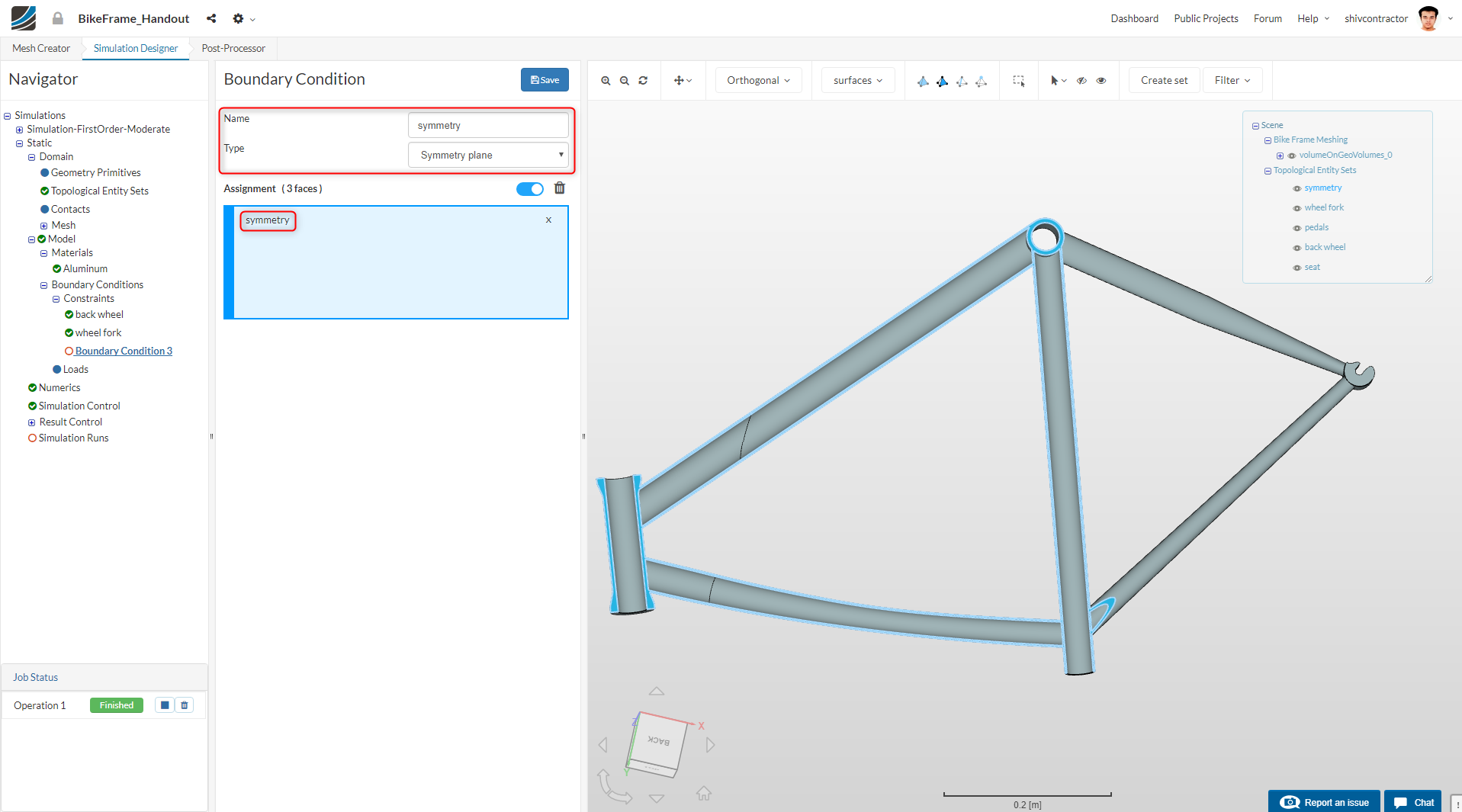
In order to reduce computation costs, the model is simplified symmetrically with a Symmetry boundary condition.
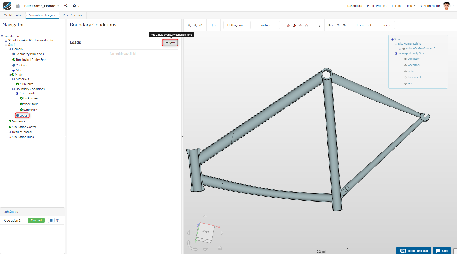
Now, we proceed to add loads. Click on Loads in the Navigator and click on New.
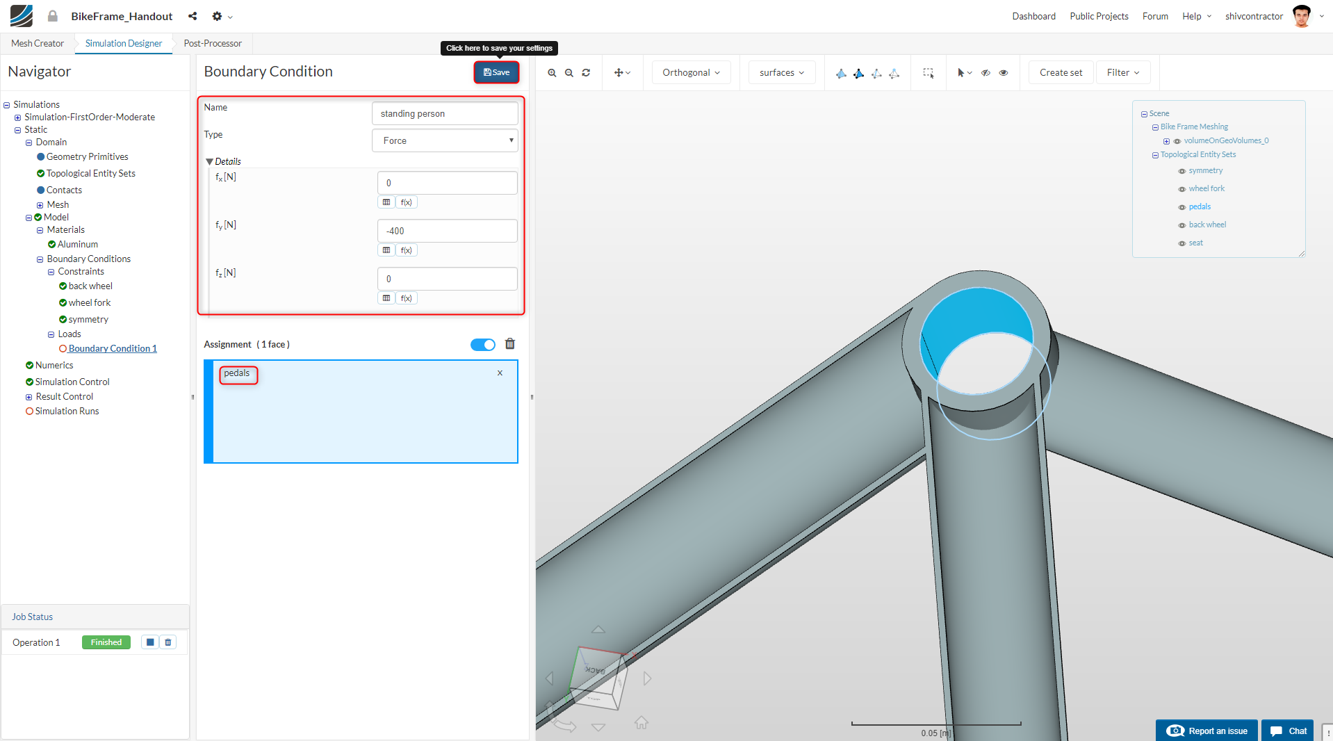
Assuming an average cyclist (Weight=81 kg) is standing on the pedals. He/she would pose a load of approximately 800 N in the -Y direction (downwards). Moreover, since we consider symmetry, the load is split in half.
fx = 0 N
fz = -800/2 = -400 N
fz = 0 N
Follow the instructions as depicted in the image below. Set an appropriate name for the force, such as standing person. Assign a force of - 400 N in the y-direction. From the panel displayed on the top right of the viewer, you can choose which component this force acts upon. In our case, this should be the pedals.
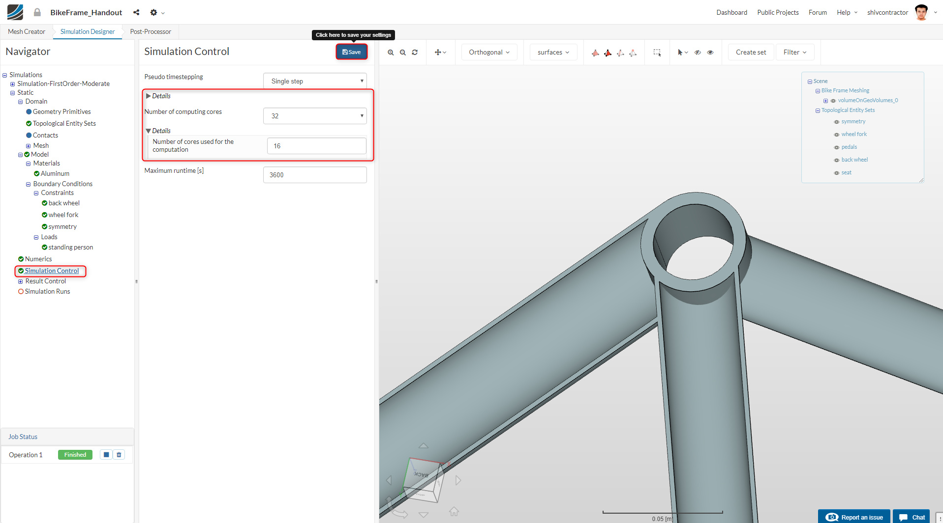
Simulation Control
Since we have used mesh refinement, a higher computational power is required for the simulation. Consequently, the Number of computing cores and Number of cores used for the computation should be increased from the default values. Set 32 for the Number of computing cores and 16 for the number of cores used for the computation.
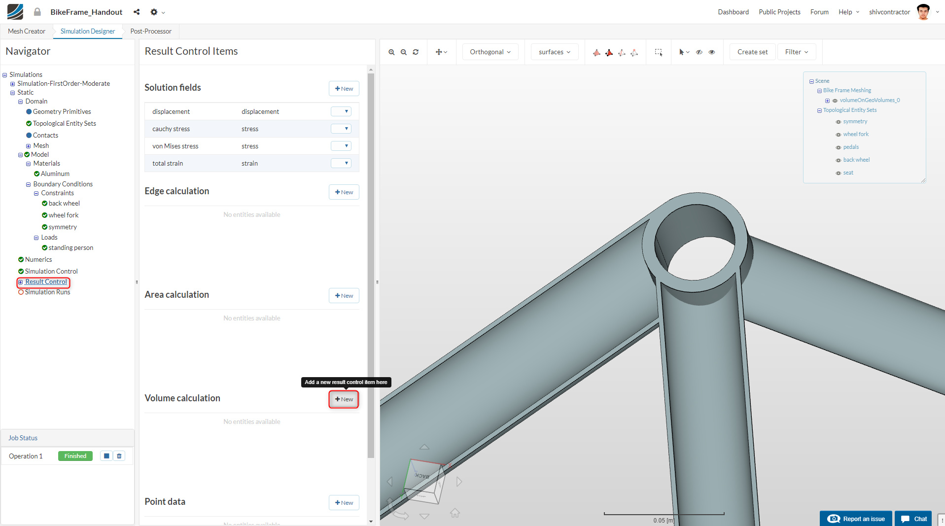
Result Control
Further, we intend to analyze solution fields such as Max-Min von Mises Stress, Displacements and Strain over the entire volume of the bike frame. Hence, it is imperative to add result control items for the volume calculation.
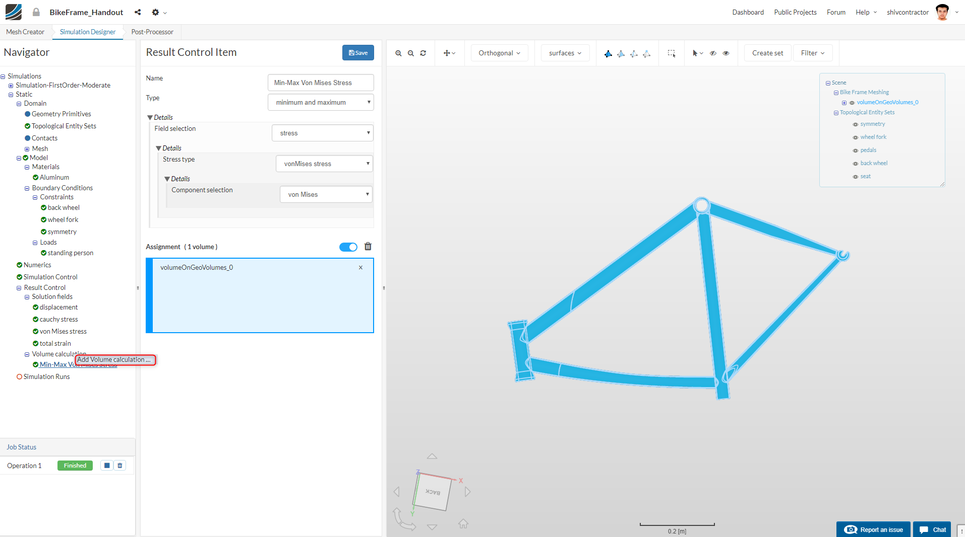
Select Result Control from the Navigator and click on New to add a new Volume Calculation item.
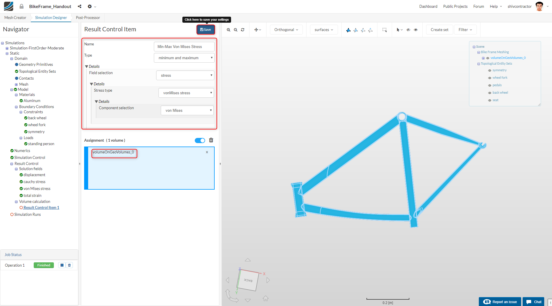
To assign the control item to the entire volume, just click once on any part of the body. The Result Control items may be set up as follows:
The Result Control items may be set up as follows:
Min-Max Von Mises Stress
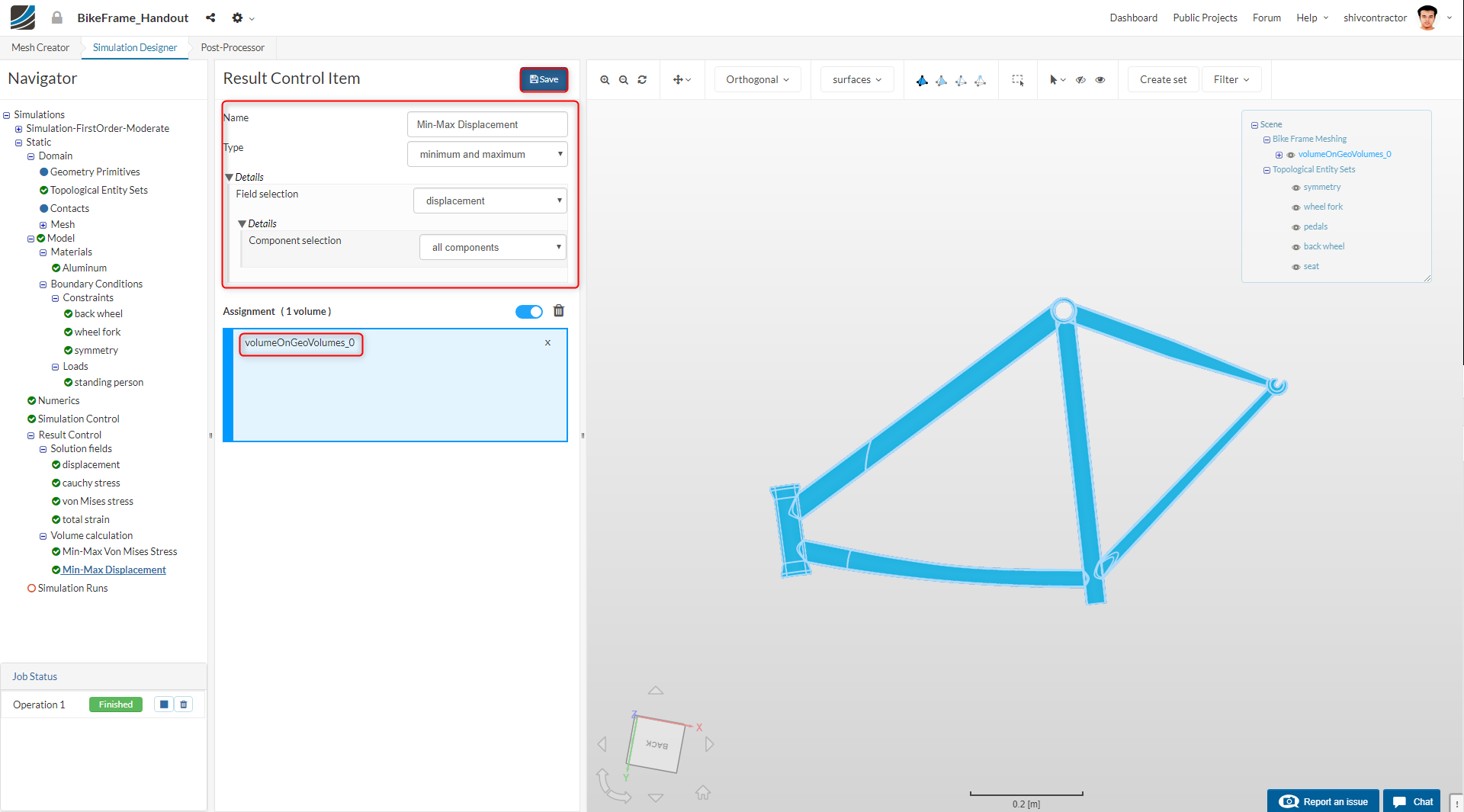
To add another volume calculation, right click on Volume Calculation and select Add Volume Calculation.
Min-Max Displacement
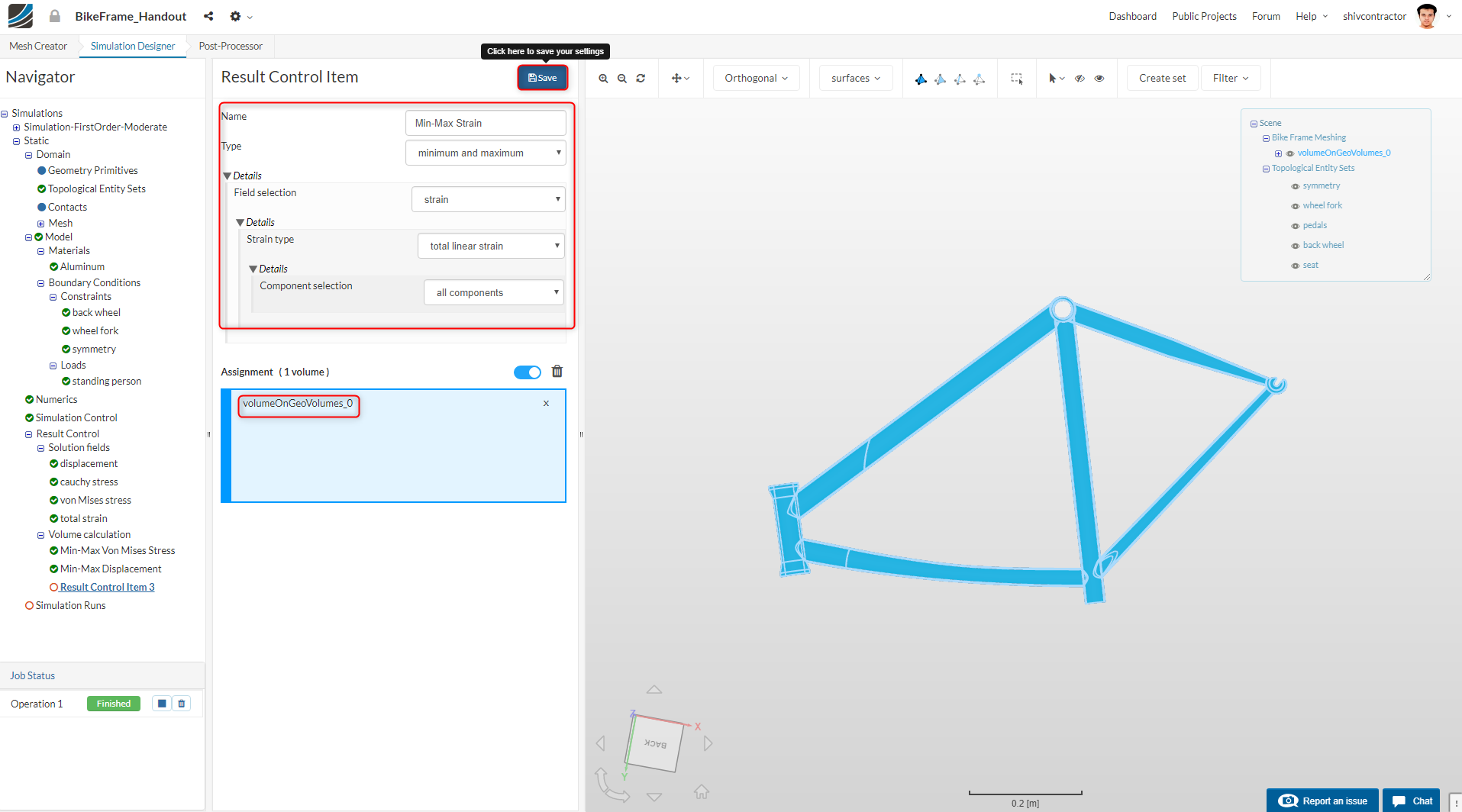
Min-Max Strain
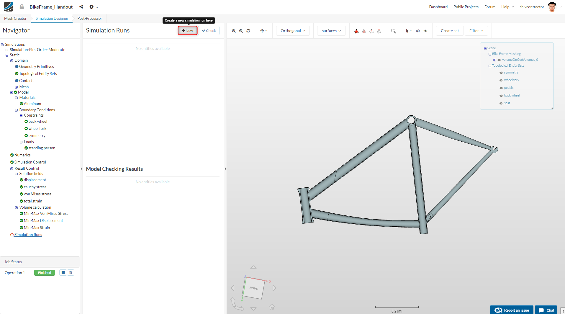
Simulation Runs
With all things set up, you can now run the simulation. In the Navigation bar, go to Simulation Runs and click on New.
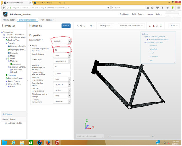
Note: You may receive the following warning when you try to create a Run:
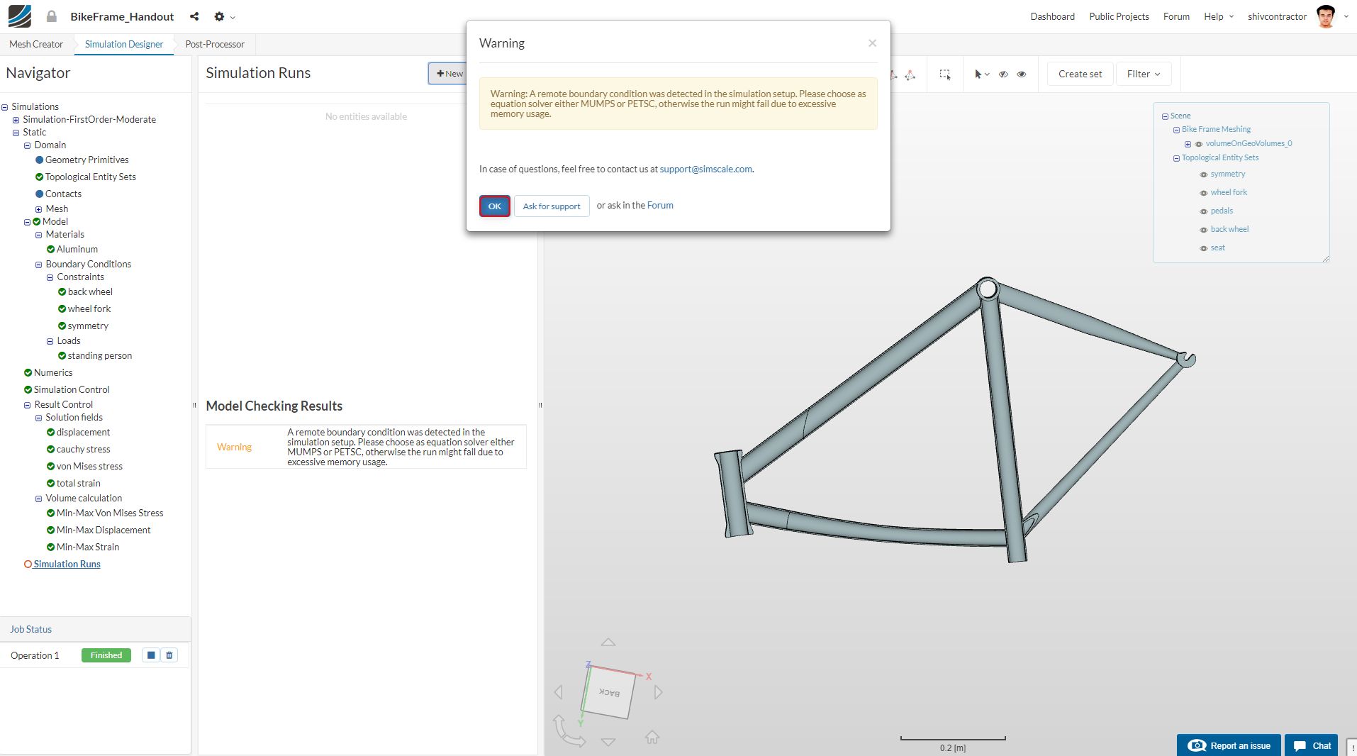
Since the solver is set to MUMPS (MUltifrontal Massively Parallel Sparse direct Solver) by default, you can click OK and continue with the simulation.
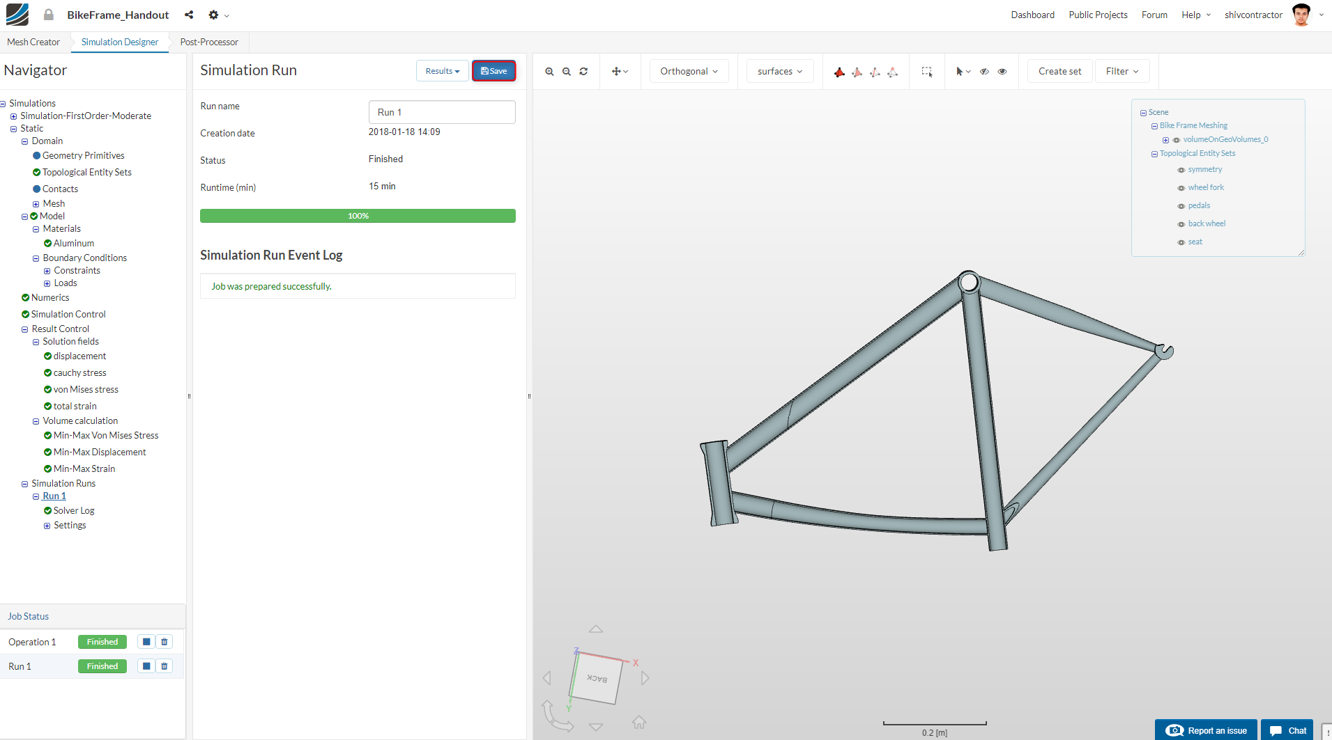
As the simulation run starts, you can track its progress in the Job Status bar on the bottom left of the display. Should there be any error/incorrect input, the simulation will fail. Don’t worry, it is only another step towards success.
Post-Processing
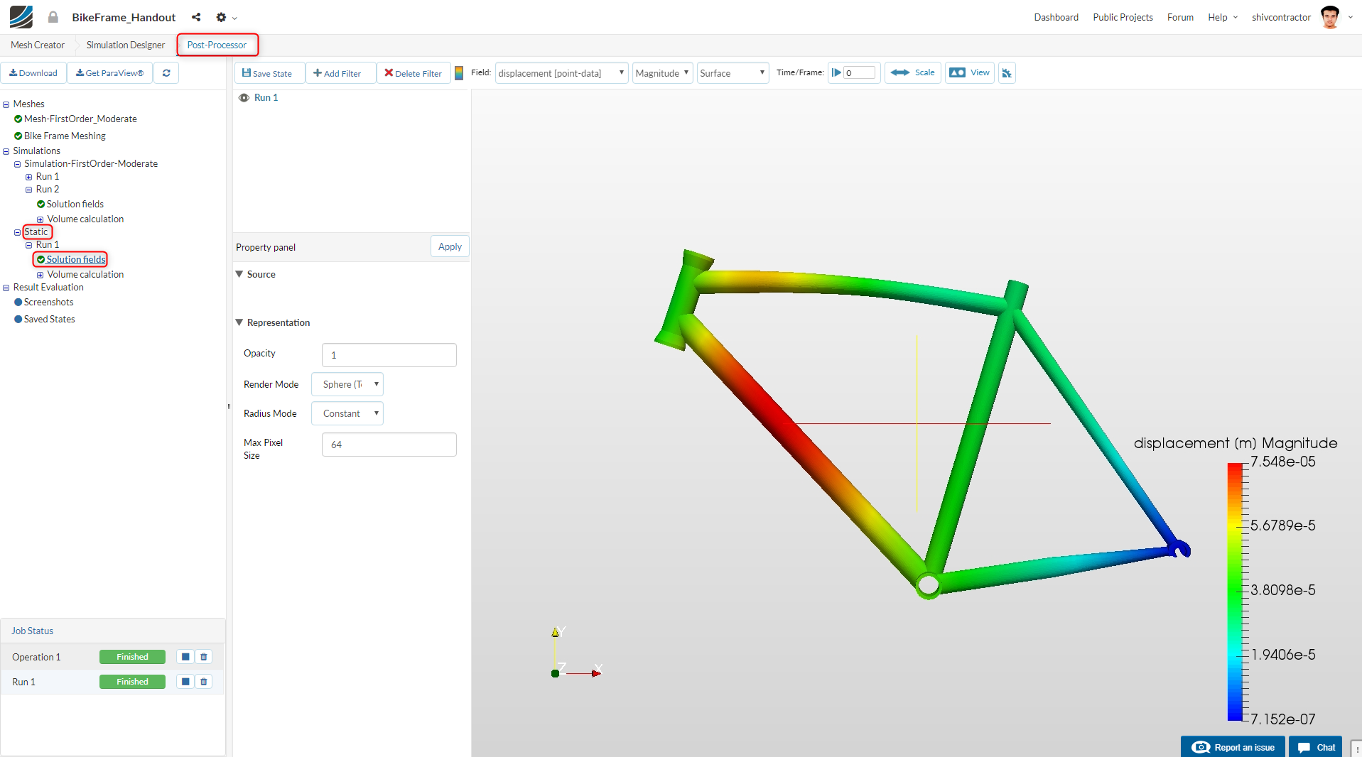
Please navigate to the Post-Processor tab.
Displacement
To visualize your result in the viewer, select it in the Navigator and click on Solution Fields. The displacement may be used to identify the regions undergoing high strain.
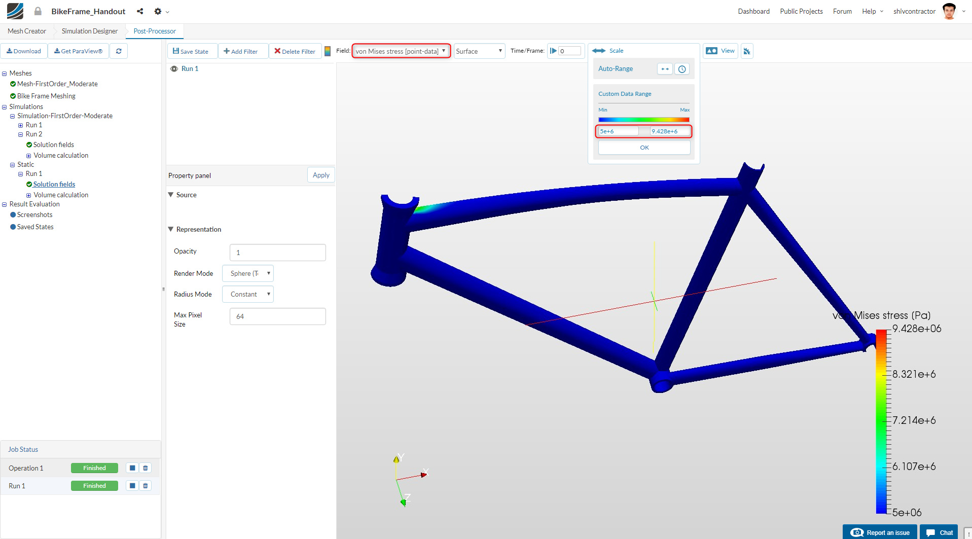
Von Mises Stress
The high-stress region may be visualized by selecting the field von Mises Stress and re-scaling the data to a suitable range.
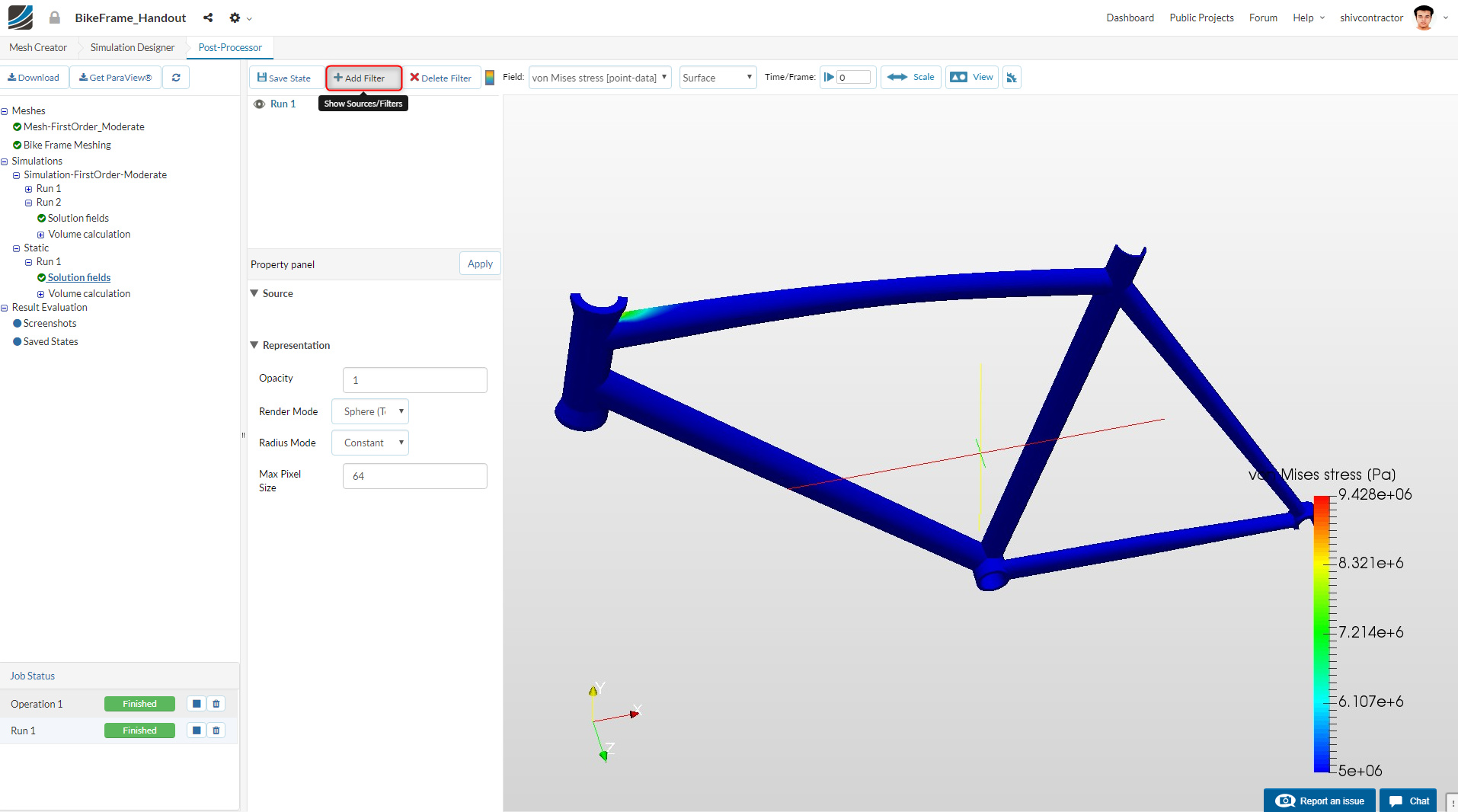
Threshold Filter
This filter enables the user to isolate the elements in the range of a particular solution field of interest.
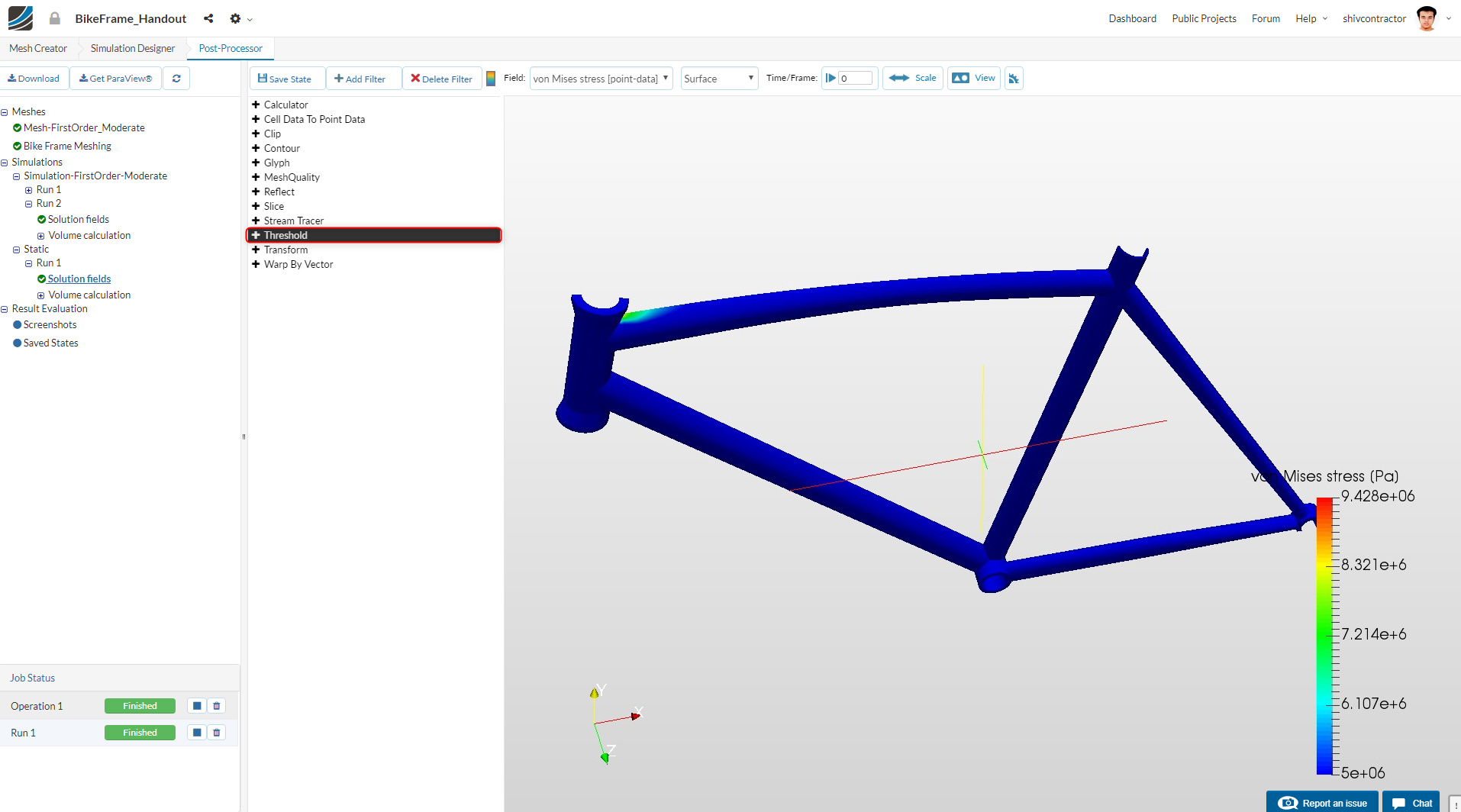
The filter may be added as follows:
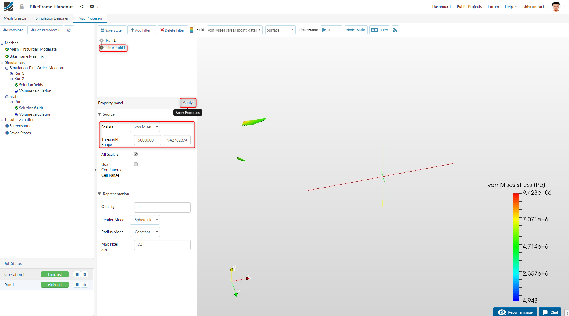
Set the quantity: Scalar to von Mises Stress and the values of the Threshold Range from 5000000 to 9427623.9
Following this, click on Apply. You will now be able to observe the von Mises Stress in the two regions as depicted below.
Plots
If you’re still curious, you can further analyze the result quantitatively for the exact values of maximum stress and displacement as follows:
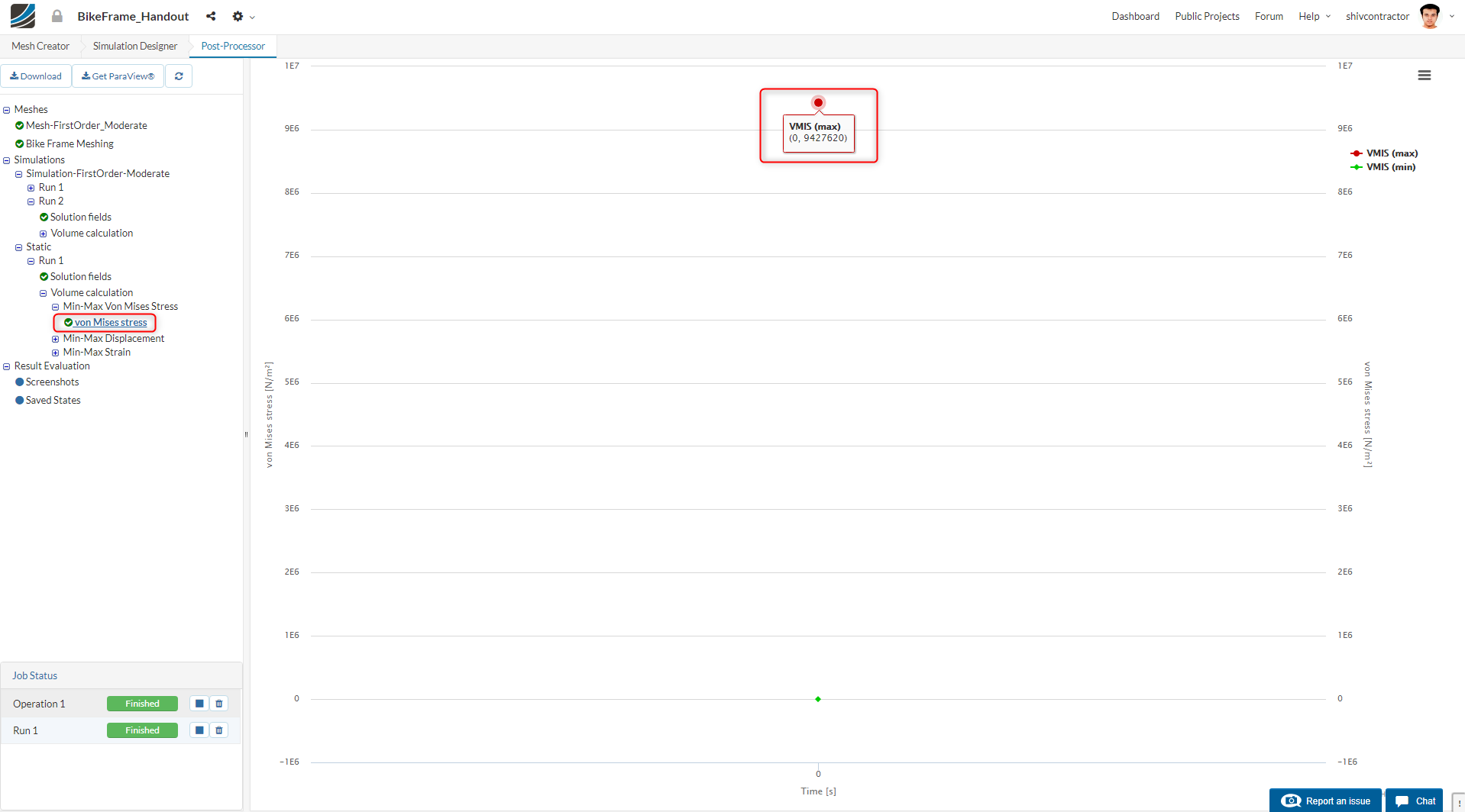
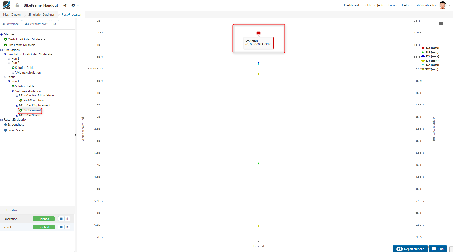
You may now compare the difference between the maximum stress and displacement values to the values from the provided simulation.
Thanks for the read and happy simulating!
References
Geometry Source: Robert Biehle