Documentation
This tutorial demonstrates how to use SimScale to run an incompressible fluid flow simulation on a centrifugal pump using rotating zones.
The complexity of this use case results from the requirement of modeling a rotating region. Such regions require additional preparation steps for both the meshing and simulation setup which we will cover in the context of this tutorial.
This tutorial teaches how to:
We are following the typical SimScale workflow:
To begin, click the button below. It will copy the tutorial project containing the geometry into your Workbench.
The following picture demonstrates the original geometry that should be visible after importing the tutorial project.
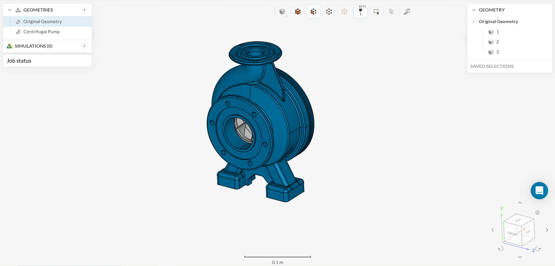
Before starting to work using SimScale’s fluid simulator analysis with rotation, we need to make sure to prepare the CAD model to be compatible with this kind of analysis. This tutorial project contains two geometries, shown in the picture below:
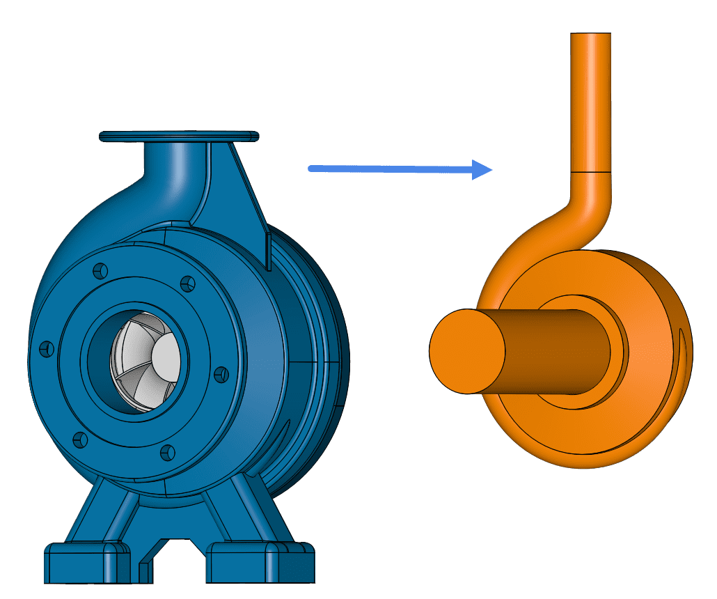
The first one (Original Geometry) consists of the actual pump and its blades. It still requires some preparation before it’s ready to use for CFD simulations.
What we need for a CFD simulation is the second geometry (Centrifugal Pump). It contains the flow region, as well as a volume representing the rotating zone. The steps to make the original geometry CFD-ready are fully described in the following article:
Make sure the Centrifugal Pump geometry is selected for this simulation project:
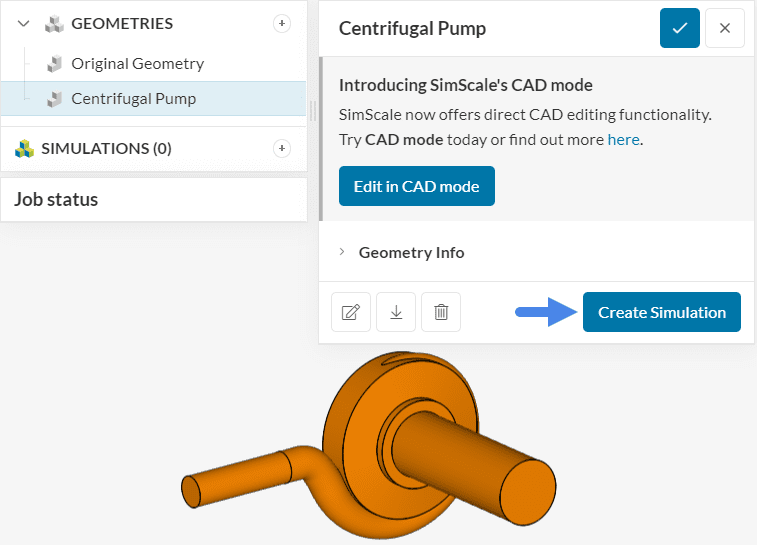
After hitting on ‘Create Simulation’, you will have several simulation types to choose from:
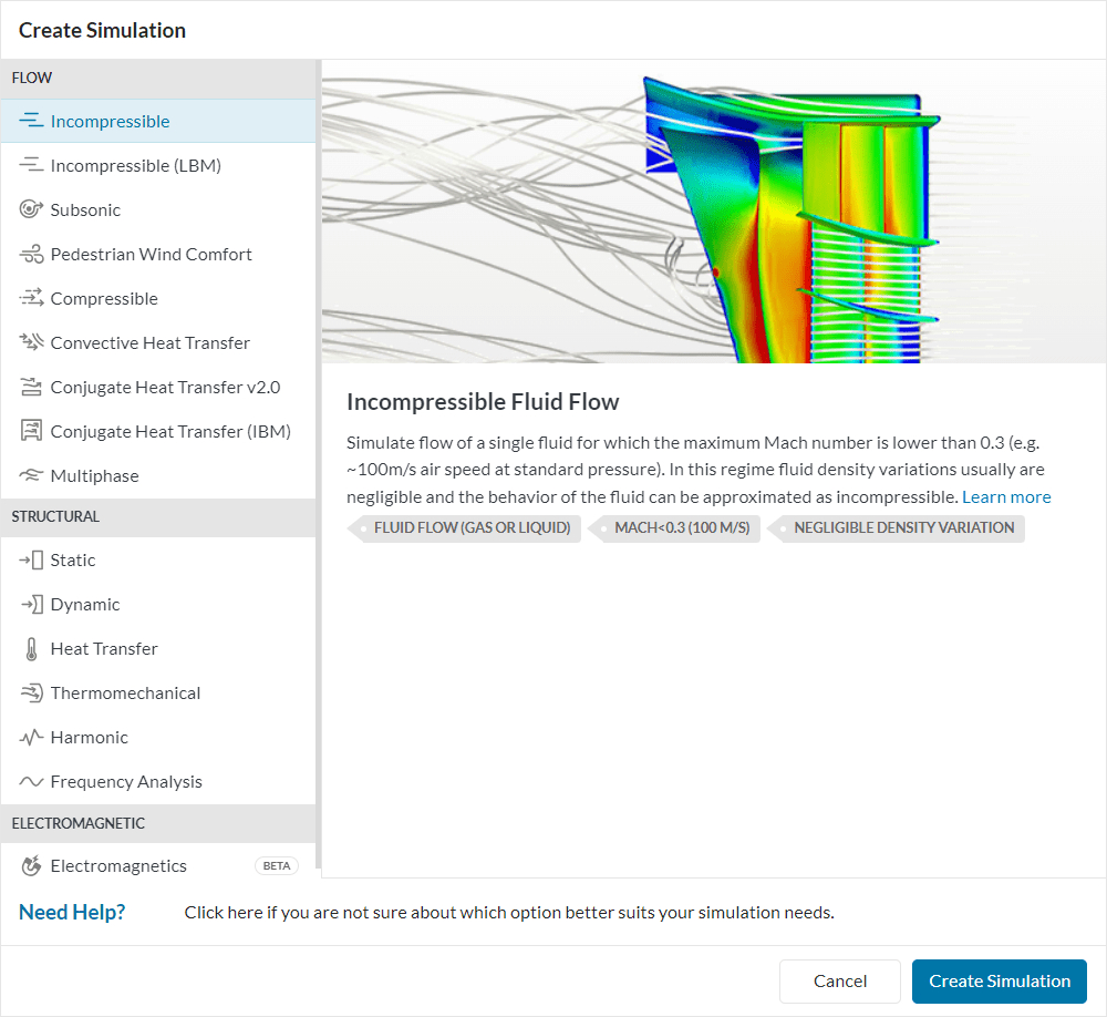
Choose ‘Incompressible’ as analysis type and ‘Create a Simulation‘.
At this point, the simulation tree will be visible in the left-hand side panel. To run the simulation, it’s necessary to configure the simulation tree entries.
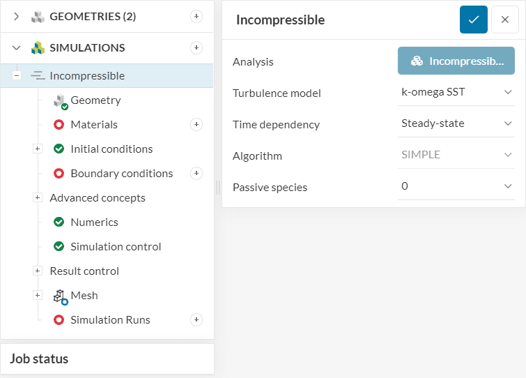
The global simulation settings remain as default, as in the figure above. With a Steady-state analysis, we will obtain the equilibrium state of the system, when the flow field no longer changes with time.
Did you know?
The k-omega SST turbulence model is commonly used in turbomachinery applications. Within the pump blades, the flow experiences separation, which is effectively captured by the k-omega SST turbulence model.
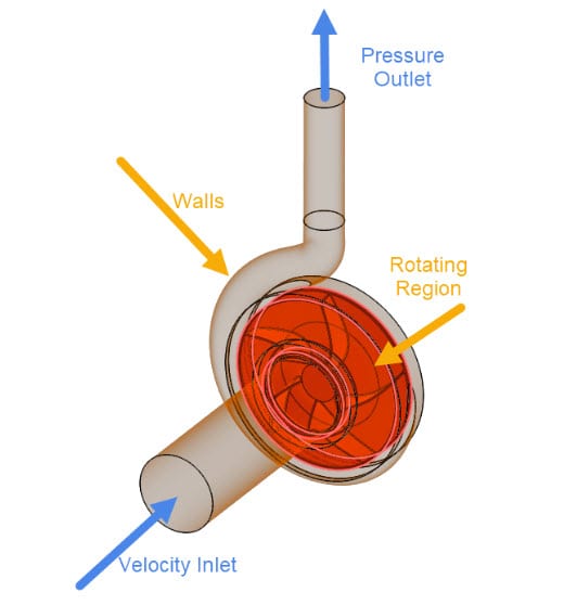
As an overview of the physics, the following picture shows the boundary conditions used in this project:
Did you know?
Velocity Inlet and Pressure Outlet is a very common combination used in CFD simulations as it often results in good stability. This combination permits flow to adjust. aiming to assure mass continuity.
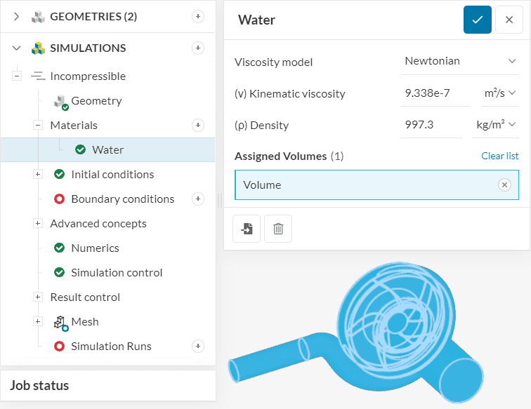
This simulation will use water as a material. Therefore click on the ‘+ button’ next to Materials. Doing this opens the SimScale fluid simulator material library as shown in the figure below:
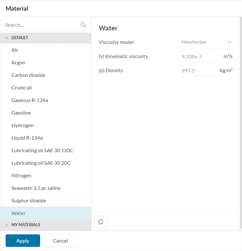
Select ‘Water’ and click ‘Apply’. A window opens up with the water properties. Keep the default values and assign them to the ‘Volume’ that represents the flow region.
In the next step, boundary conditions need to be assigned as in figure 7. We have a velocity inlet, a pressure outlet, walls, and a rotating zone.
a. Velocity Inlet
After hitting the ‘+ button’ next to Boundary conditions, a drop-down menu will appear, where one can choose between different boundary conditions.
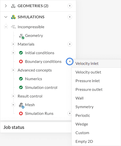
After selecting ‘Velocity inlet’, you can specify the velocity configuration and assign faces. Please proceed as follows:
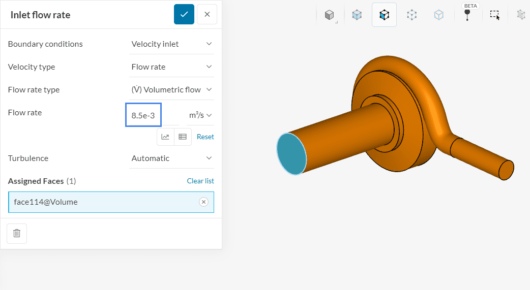
With these settings, a volumetric flow rate of ‘8.5e-3’ \(m^3/s\) enters the domain through the inlet.
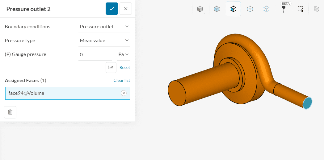
b. Pressure Outlet
Create a new boundary condition, this time a ‘Pressure outlet’. Make sure (P) Gauge Pressure is set to ‘Mean value = 0’.
c. Wall
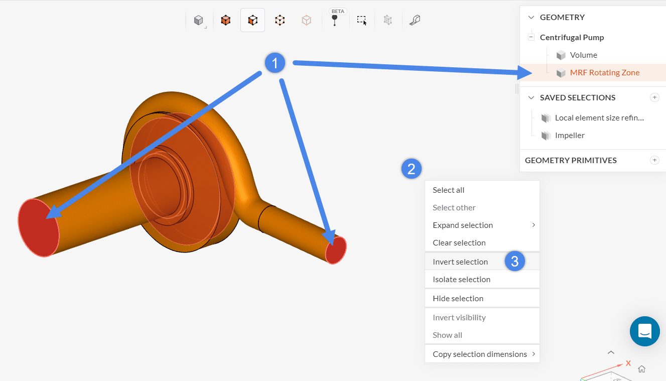
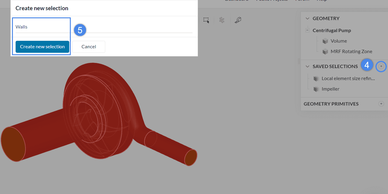
All solid walls should receive a no-slip condition. We can make use of SimScale’s quick selection tools to save time. A Saved selection will be created, as this set of faces will be used again during the setup.
Please follow the following steps:
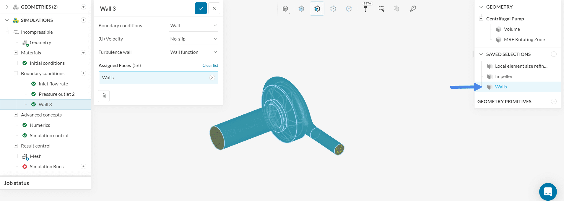
Afterward, create a ‘Wall’ boundary condition and assign it to the newly created saved selection.
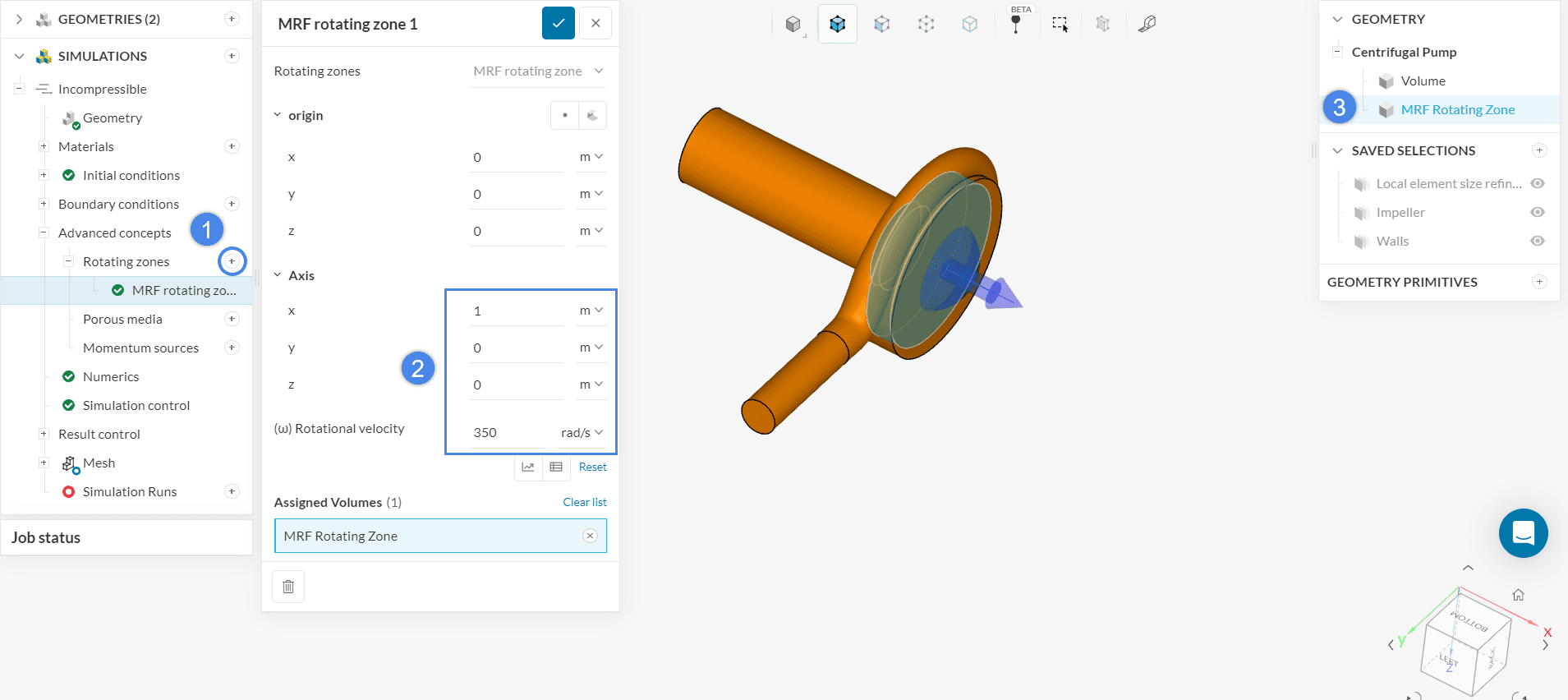
In the simulation tree, please expand Advanced concepts. Click on the ‘+ button’ next to Rotating zones and select an ‘MRF Rotating Zone’. Define the MRF zone as shown:
Did you know?
MRF Rotating zones are chosen in this simulation because we are running a steady-state simulation.
If we were calculating a transient problem, we would need to choose AMI Rotating Zone.
This article provides more information about the difference between MRF and AMI Rotating Zones.
Don’t worry about the Numerics settings, as their default values are optimized according to the chosen analysis type, hence valid for the majority of simulations. If you are a simulation expert, however, you can have a look at them and change the settings as you like.
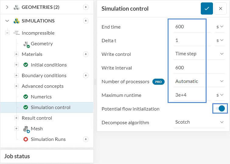
Under the Simulation control settings, enable ‘Potential flow initialization’, which enhances the stability for velocity-driven flows, especially in early iterations. The new Maximum runtime is ‘30000’ seconds, and both End time and Write interval will be ‘600’ iterations.
Result control allows you to observe the convergence behavior at specific locations in the model during the calculation process. Hence it is an important indicator to evaluate the quality and reliability of the results.
For this simulation, please set a ‘Forces and moments’ control to the impeller as demonstrated in the picture below:
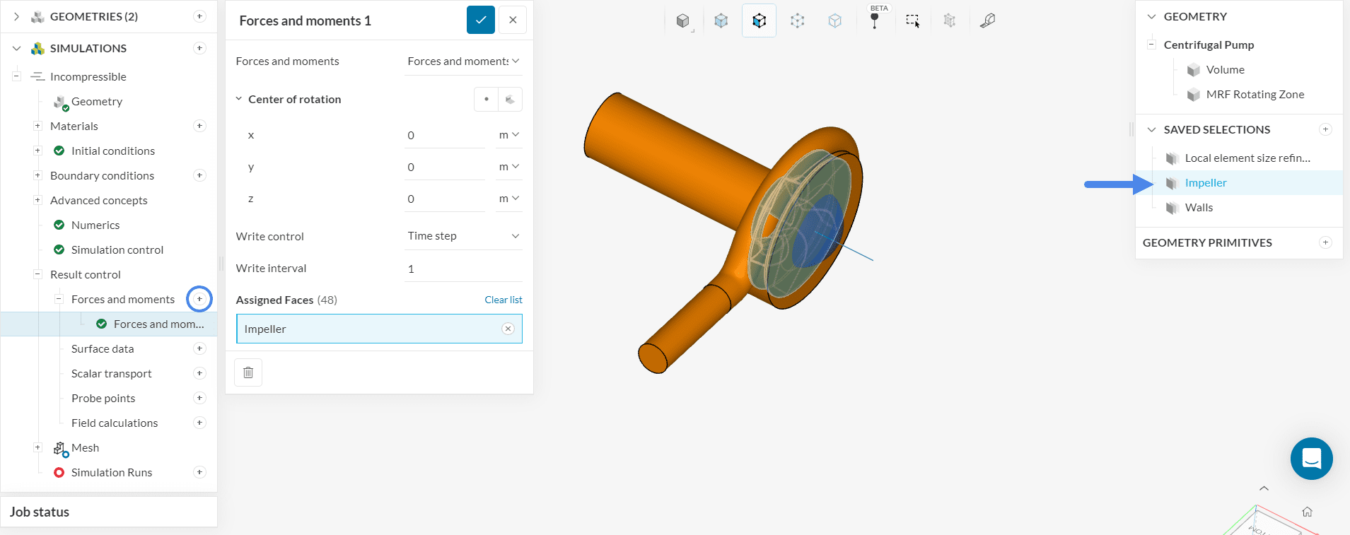
To save time, there’s a pre-saved saved selection for the Impeller surfaces. Finally, click on the ‘+’ button next to Surface data. Create an ‘Area average’ for the inlet and another one for the outlet:
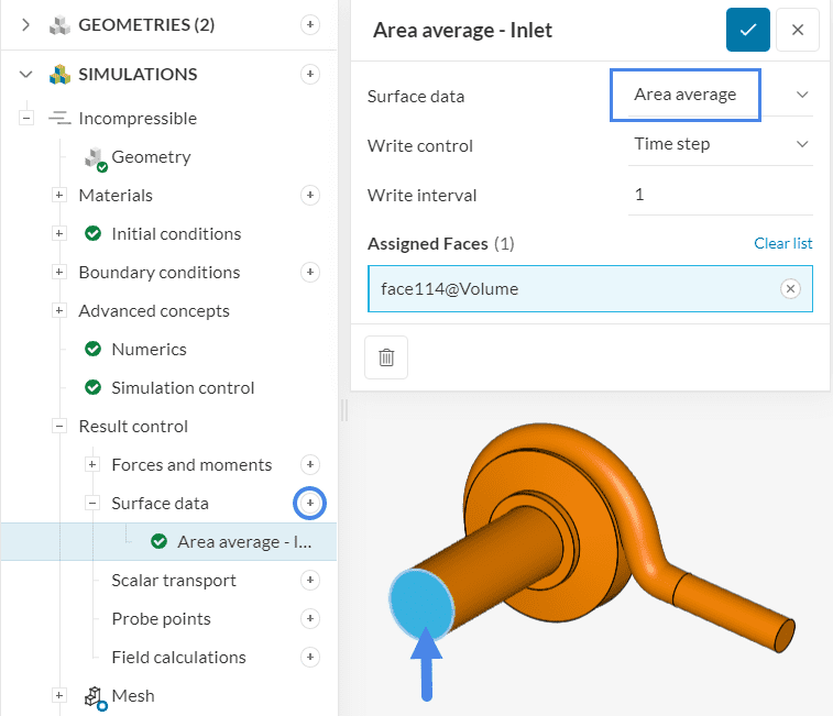
Create another area average result control, this time for the outlet.
To create the mesh, we recommend using the Standard algorithm, which is a good choice in general as it is quite automated and delivers good results for most geometries.
In this tutorial, the global simulation settings will remain as default, and a local refinement will be applied to the regions of interest.
Did you know?
It’s necessary to define cell zones whenever we want to apply a specific property, such as a rotating motion, to a subset of cells.
The standard mesher automatically creates the necessary cell zones whenever Physics-based meshing is enabled. Since we are using physics-based meshing in this tutorial, the algorithm will take care of the cell zone definition.
If you are using a different mesher, you can learn alternative ways to define a cell zone on the rotating zones documentation page.
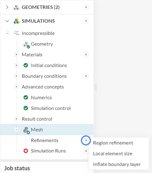
To create a new refinement, click on the ‘+ button’ next to Refinements. Afterward, choose ‘Local element size’ from the drop-down window.
The Maximum edge length should be ‘7e-4’ meters, applied to the Local element size refinement saved selection.
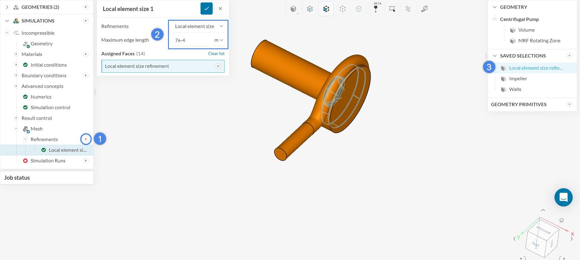
With this refinement, you will have better control over the cell size in the regions of interest.
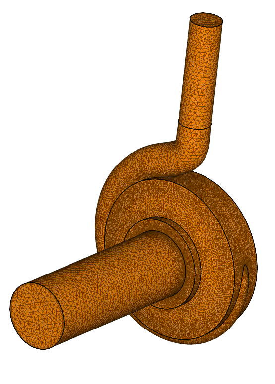
Now you can navigate to the ‘Mesh’ entry in the simulation tree and hit the ‘Generate’ button. After a few minutes you will receive the following mesh:
Did you know?
Generating meshes with good quality metrics is important. These meshes increase the stability of the simulation runs and also increase the confidence level in the results.
For a complete overview of mesh quality and its importance in CFD simulations, make sure to visit this documentation page.
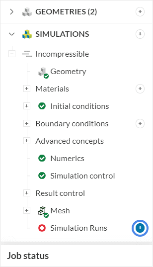
Now you can ‘Start’ the simulation. While the results are being calculated you can already have a look at the intermediate results in the post-processor by clicking on ‘Solution Fields’. They are being updated in real-time!
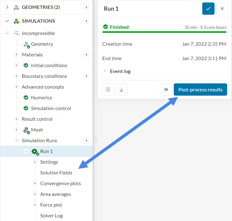
It takes roughly one hour for the simulation to finish. In the reference project, we calculated a few more steps, to ensure convergence, that’s why it says 105 min in the figure below. However, fewer steps are sufficient and you can save some core hours.
Did you know?
With SimScale, it’s easy to get the pump curve for your geometry. You can run multiple simulations in parallel, only changing the flow rate (in the velocity inlet boundary condition).
For more information about pump curves, please check out this blog post.
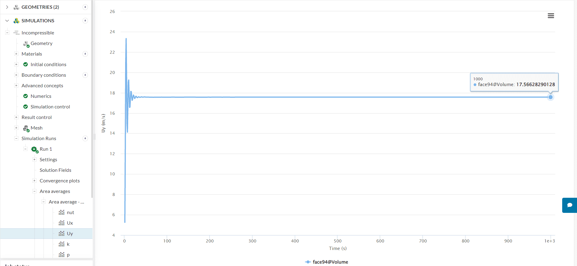
With the previously set result controls, it’s possible to assess convergence. As the iterations go on, key parameters are expected to stop changing. At this point, the simulation is considered converged.
So what are the key parameters? For a centrifugal pump simulation, the velocity at the outlet, the pressure at the inlet, and forces onto the impeller are parameters of interest. For example, let’s have a look at velocity at the outlet:
Also, make sure to check the convergence plots to see residual levels. Smaller residuals indicate a more tightly converged solution. This article gives more insight into convergence in CFD simulations.
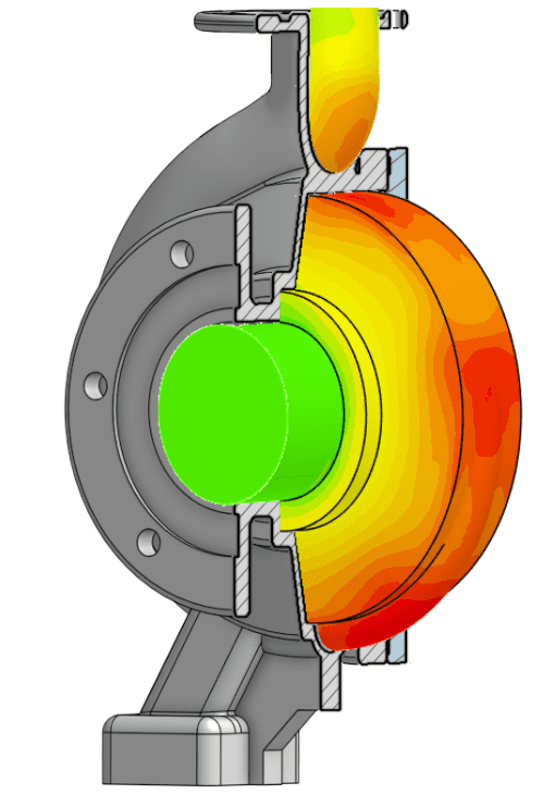
SimScale has a built-in post-processing environment, which can be accessed by clicking on ‘Solution Fields’ or ‘Post-process results’, as in figure 24. First, let’s visualize the pressure levels on the blades:
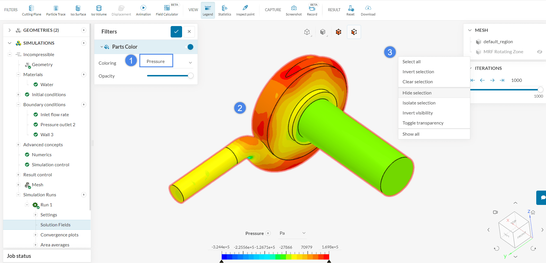
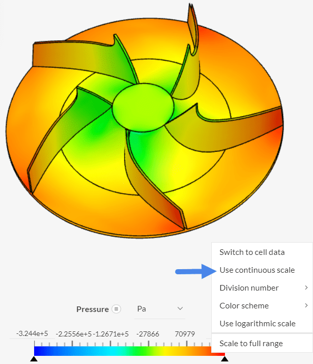
After hiding the first set of faces, you may have to hide more internal faces before the blades are fully visible. At this stage, right-click on the legend and select ‘Use continuous scale’ to make the color scheme smoother:
To get a better understanding of what is going on inside the pump, proceed to add a ‘Cutting Plane’ filter:
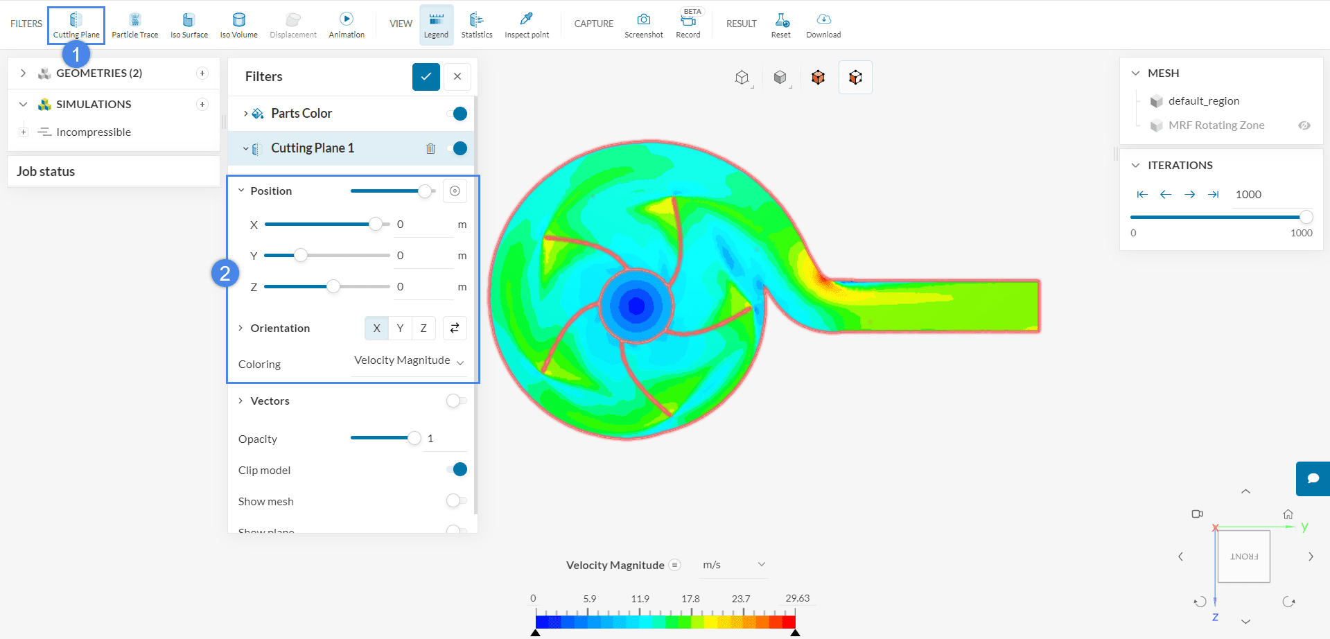
You can also toggle on the vectors to check the flow direction of the field in different areas:
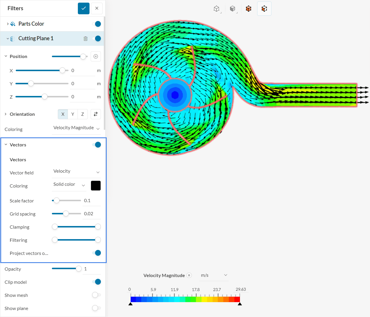
Near the edges of the blades, the acceleration of the flow can be distinguished due to the representation with a warmer color compared to its surroundings. Other configurations for the cutting plane will give you additional information. For instance, you can change the Orientation to ‘Y’
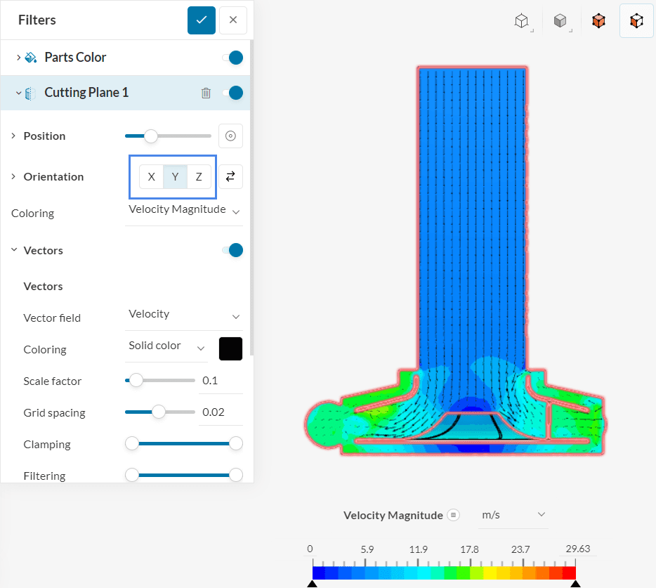
With this configuration, you can observe the flow pattern around the blades from a different perspective.
Analyze your results with the SimScale post-processor. Have a look at our post-processing guide to learn how to use the post-processor.
Note
If you have questions or suggestions, please reach out either via the forum or contact us directly.
Last updated: October 9th, 2023
We appreciate and value your feedback.
Sign up for SimScale
and start simulating now