Documentation
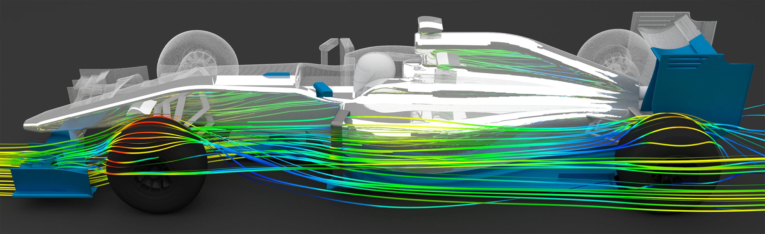
Computational Fluid Dynamics (CFD) is the process of mathematically predicting physical fluid flow by solving the governing equations using computational power.
When an engineer is tasked with designing a new product, e.g. a winning race car for the next race season, aerodynamics plays an important role in the overall performance of the design. That said, aerodynamic performance is not easily quantifiable during the concept phase.
Traditionally, the only way for an engineer to optimize his/her design is to conduct physical tests on product prototypes. With the rise of computers and ever-growing computational power (thanks to Moore’s law), the field of CFD has become a commonly applied tool for predicting real-world physics.
In a CFD software analysis, fluid flow and its associated physical properties, such as velocity, pressure, viscosity, density, and temperature, are calculated based on defined operating conditions. In order to arrive at an accurate, physical solution, these quantities are calculated simultaneously.
Every CFD tool, both commercial and/or open source, uses a mathematical model and numerical method to predict the desired flow physics. The most common CFD tools are based on the Navier-Stokes (N-S) equations. While the bulk of the terms in the Navier-Stokes equations remains constant, more terms can be added or removed based on the physics. For example, if heat transfer, phase change, or chemical reactions need to be considered, more terms will be introduced into the governing equations.
It is very important that the proper operating conditions, numerical methods, and physics are considered in order to conduct an accurate and successful CFD analysis. If this is done correctly, performance insights can be obtained quickly that will result ultimately in a better performing and more efficient final product.
From antiquity to the present, humankind has been eager to explain their observations of fluid flow. So, how old is CFD? The field of CFD has one big disadvantage: it is extremely computationally expensive, and therefore progress could not be made until computing power made significant improvements in cost and performance. Until this happened, scientists and engineers focused primarily on improving mathematical models and numerical methods which would reduce computational costs.
The brief story of Computational Fluid Dynamics can be understood below:
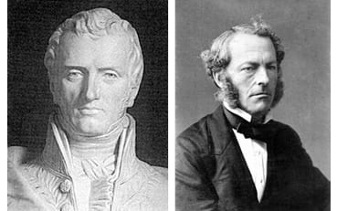
The central mathematical description for all theoretical fluid dynamics models is given by the Navier-Stokes equations, which describe the motion of viscous fluid domains. The history of their discovery is quite interesting.
It is a bizarre coincidence that the famous equation of Navier-Stokes has been generated by Claude-Louis Navier (1785-1836) and Sir George Gabriel Stokes (1819-1903), who had never met. At first, Claude-Louis Navier conducted studies on a partial section of equations up until 1822. Later, Sir George Gabriel Stokes adjusted and finalized the equations in 1845\(^9\).
The main structure of thermo-fluids examination is directed by governing equations that are based on the conservation law of fluid’s physical properties. The basic equations are the three laws of conservation\(^{10,11}\):
These principles state that mass, momentum, and energy are stable constants within a closed system. In short, everything must be conserved.
The investigation of fluid flow with thermal changes relies on certain physical properties. The three unknowns which must be obtained simultaneously from these three basic conservation equations are the velocity \(\vec{v}\), pressure \(p\) and temperature \(T\). Yet \(p\) and \(T\) are considered the two required independent thermodynamic variables.
The final form of the conservation equations also contains four other thermodynamic variables; density \(\rho\), enthalpy \(h\), viscosity \(\mu\), and thermal conductivity \(k\); the last two of which are also transport properties. These four properties are uniquely determined by the value of \(p\) and \(T\).
Fluid flow should be analyzed to know \(vec{v}\), \(p\) and \(T\) throughout every point of the flow regime. Furthermore, the method of fluid flow observation based on kinematic properties is a fundamental issue. The movement of fluid can be investigated with either Lagrangian or Eulerian methods.
This missile example precisely explains the two methods.
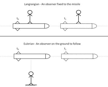
Lagrangian: We take up every point at the beginning of the domain and trace its path until it reaches the end.
Eulerian: We consider a window (Control Volume) within the fluid and analyze the particle flow within this volume.
The equation for the Conservation of Mass is specified as:
$$ \frac{Dρ}{Dt} +\rho (\nabla \cdot \vec{v}) =0 \tag{3}$$
where \(\rho\) is the density, \(\vec{v}\) the velocity and \(\nabla\) the gradient operator.
$$ \vec{\nabla} = \vec{i} \frac{\partial}{\partial x} + \vec{j} \frac{\partial}{\partial y} + \vec{k} \frac{\partial}{\partial z} \tag{4}$$
If the density is constant, the flow is assumed to be incompressible and the continuity equation reduces to:
$$ \frac{D\rho}{Dt} = 0 \rightarrow \nabla \cdot \vec{v} = \frac{\partial u}{\partial x} + \frac{\partial v}{\partial y} + \frac{\partial w}{\partial z} = 0 \tag{5}$$
Conservation of Momentum which can be referred to as the Navier-Stokes Equation is given by:
$$ \overbrace{\frac{\partial}{\partial t} (\rho \vec{v})}^{I} + \overbrace{\nabla \cdot (\rho \vec{v} \vec{v})}^{II}= \overbrace{-\nabla p}^{III} + \overbrace{\nabla \cdot \left(\overline{\overline{\tau}}\right)}^{IV} + \overbrace{\rho \vec{g}}^{V} \tag{6}$$
where \(p\) is static pressure, \(\overline{\overline{\tau}}\) is viscous stress tensor and \(\rho \vec{g}\) is the gravitational force per unit volume. Here, the roman numerals denote:
I: Local change with time
II: Momentum convection
III: Surface force
IV: Diffusion term
V: Mass force
Viscous stress tensor \(\overline{\overline{\tau}}\) can be specified as below in accordance with Stoke’s Hypothesis:
$$ \tau_{ij} = \mu \frac{\partial v_i}{\partial x_j} + \frac{\partial v_j}{\partial x_i} – \frac{2}{3}(\nabla \cdot \vec{v}) \delta_{ij} \tag{7}$$
If the fluid is assumed to be incompressible with constant viscosity coefficient \(\mu\) the Navier-Stokes equation simplifies to:
$$ \rho \frac{D\vec{v}}{Dt} = -\nabla p + \mu \nabla^2 \vec{v} + \rho \vec{g} \tag{8}$$
Conservation of Energy is the first law of thermodynamics which states that the sum of the work and heat added to the system will result in the increase of the energy in the system:
$$ dE_t=dQ + dW \tag{9}$$
where \(dQ\) is the heat added to the system, \(dW\) is the work done on the system and \(dE_t\) is the increment in the total energy of the system. One of the common types of an energy equation is:
$$ \rho \left[\overbrace{\frac{\partial h}{\partial t}}^{I} + \overbrace{\nabla \cdot (h\vec{v})}^{II} \right] = \overbrace{-\frac{\partial p}{\partial t}}^{III} + \overbrace{\nabla \cdot (k\nabla T)}^{IV} + \overbrace{\phi}^{V} \tag{10}$$
I: Local change with time
II: Convective term
III: Pressure work
IV: Heat flux
V: Source term
The Mathematical model merely gives us interrelation between the transport parameters which are involved in the whole process, either directly or indirectly. Even though every single term in those equations has a relative effect on the physical phenomenon, changes in parameters should be considered simultaneously through the numerical solution, which comprises differential equations, vector-, and tensor notations.
A PDE comprises more than one variable and is denoted with “\(\partial\)”. If the derivation of the equation is conducted with “\(d\)”, these equations are called Ordinary Differential Equations (ODE) that contain a single variable and its derivation. The PDEs are implicated to transform the differential operator (\(\partial\)) into an algebraic operator in order to get a solution. Heat transfer, fluid dynamics, acoustic, electronics and quantum mechanics are all fields in which PDEs are highly used to generate solutions.
Example of ODE:
$$ \frac{d^2 x}{dt^2} = x \rightarrow x(t) \quad \text{where T is the single variable} \tag{11}$$
Example of PDE:
$$ \frac{\partial f}{\partial x} + \frac{\partial f}{\partial y} = 5 \rightarrow f(x,y) \quad \text{where both x and y are the variables} \tag{12}$$
What is the significance of PDEs in seeking a solution to governing equations? To answer this question, we initially examine the basic structure of some PDEs to create connotation. For instance:
$$ \frac{\partial^2 f}{\partial x^2} + \frac{\partial^2 f}{\partial y^2} = 0 \rightarrow f(x,y) \rightarrow \text{Laplace Equation} \tag{13}$$
A quick comparison between equation (5) and equation (13) specifies the Laplace part of the continuity equation. What is the next step? What does this Laplace analogy mean? To start solving these enormous equations, the next step comes through discretization to ignite the numerical solution process.
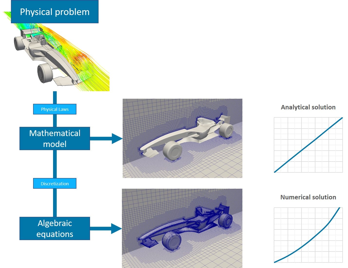
The numerical solution is a discretization-based method used to obtain approximate solutions to complex problems that cannot be solved with analytic methods. As seen in Figure 4, solution processes without discretization merely give you an analytic solution which is exact but simple.
Moreover, the accuracy of the numerical solution highly depends on the quality of the discretization. Broadly used discretization methods might be specified, such as finite difference, finite volume, finite element, spectral (element) methods and boundary element.
Multitasking is one of the plagues of the century that generally ends up with procrastination or failure. Therefore, having planned, segmented and sequenced tasks is much more appropriate for achieving goals: this has also been working for CFD.
In order to conduct an analysis, the solution domain is split into multiple sub-domains, which are called cells. The combination of these cells in the computational structure is named mesh.
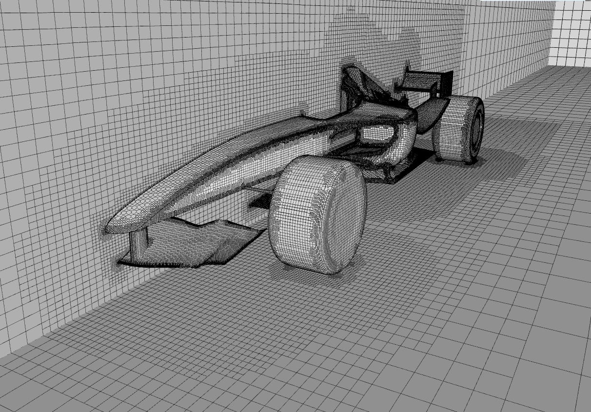
Meshing is the process of discretization of the domain into small cells or elements to apply the mathematical model under the assumption of linearity pertaining to each cell. This means that we need to ensure that the behavior of the variables that need to be solved can be assumed linear within each cell. This requirement also implies that a finer mesh is needed for areas where the physical properties to be predicted are suspected to be highly mercurial. To know more about meshing, readers are highly encouraged to read “What is a mesh?“
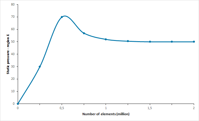
Errors due to mesh are a common issue that results in inaccurate solutions or outright failure of the simulation. This can happen because the mesh is too coarse and flow physics are not captured within an area of large, coarse cells. Because of this, a mesh independence study needs to be carried out to ensure the mesh is not having a tangible impact on the solution. An example of a mesh independence study can be defined as below:
By doing this, errors based on the mesh structure can be eliminated and the optimum number of elements may be achieved to make computation an efficient process. Figure 6 looks into static pressure change at imaginary region X through the increase in the number of mesh elements. According to Figure 6, around 1,000,000 elements would have been sufficient to conduct a reliable study.
Creating a sculpture requires a highly talented artist with the ability to imagine the final product from the beginning. That said, a sculpture is a simple piece of rock in the beginning but might become an exceptional artwork in the end. The process of gradually carving away material is central to obtaining the desired final shape.
CFD also has a similar process that relies on gradually changing results which eventually land on a final solution. During a CFD analysis, an initial guess is used as a starting point; is analogous to the stone block an artist starts with. Through numerical iteration, the solution field morphs from an initial guess into a final, persisting flow field. Keep in mind that while numerical iterations are responsible for arriving at a final solution, the result accuracy is still completely dependent on the mesh for an accurate solution.
Convergence is a paramount issue for computational analysis. The movement of fluid has a non-linear mathematical model with various complex models such as turbulence, phase change, and mass transfer; and convergence is heavily influenced by them. Apart from the analytical solution, the numerical solution goes through an iterative scheme in which results are obtained by the reduction of errors among previous stages. The differences between the last two solutions specify the error. When the absolute error is descending, the reliability of the result increases, and the result converges towards a stable solution.
The solving should continue, iterating further and further until the solution field stops changing. This is true with both steady-state and transient simulations. For transient simulations, convergence has to be obtained at each time step as if it was a steady-state simulation.
The residuals of equations, like stone leftovers from a sculpture, change with each iteration. As iterations get down to a threshold value, convergence is achieved. This is analogous to an artist removing the final small piece of stone from a sculpture. A few more key facts about convergence:
Join SimScale today!
All the applications mentioned below can be simulated within the SimScale platform. If you want to solve and visualize the equations described earlier in the form of colourful and informative results, sign up with our community plan.
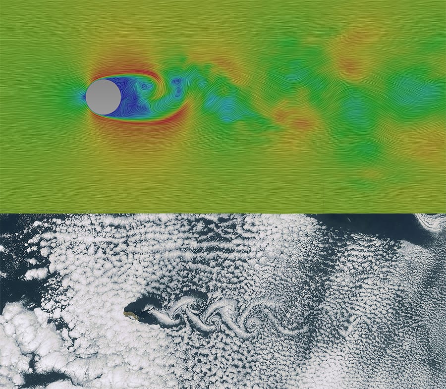
CFD can be used in every possible application that involves fluid flow. For example, flow over a cylinder is a classic academic example that is taught in university-level fluids courses. The same phenomenon can be observed in the movement of clouds in the atmosphere, as seen in Figure 7.
If compressibility becomes a non-negligible factor, this type of analysis helps you to find solutions for compressible flows in a very robust and accurate way. One example would be a Large Eddy Simulation of flow around a cylinder.
Depending on flow properties such as density, viscosity, and velocity, flow can be characterized as either laminar or turbulent. Most commercial applications of flow are generally turbulent; however, there are exceptions. For example, natural convection flow from a warm light is considered laminar flow. Turbulent simulations are slightly more computationally expensive as there are more terms in the governing equations. This valve is one example of turbulent flow analysis.
Mass transport simulations include smoke propagation, passive scalar transport, or gas modeling. SimScale uses OpenFOAM solvers to analyze these kinds of simulations.
Heat exchanger simulations are an example of one possible application.
Interested in reading more CFD-related content?
CFD tools vary in accordance with the mathematical models, numerical methods, computational equipment, and post-processing tools used alongside them. For example, a single physical phenomenon could be modeled with two completely different mathematical approaches, numerical methods, and computational hardware.
That said, over the past decade, several codes/methods have become more common due to their robustness. SimScale currently uses a mix of both open-source and commercially licensed software solutions. OpenFOAM is perhaps the most well-known open-source CFD software that exists today. SimScale leverages OpenFOAM as well as other proprietary CFD solvers.
Given the cloud-based nature of SimScale, a wide range of applications related to laminar, turbulent, incompressible, compressible, and multiphase flow and heat transfer physics can seamlessly be explored from a web browser. By using SimScale, an engineer can leverage dozens of tightly integrated numerical solvers, meshers, and visualization technologies that result in a capable end-to-end CAE solution.
References
Last updated: December 7th, 2023
We appreciate and value your feedback.
What's Next
What is Buoyancy?Sign up for SimScale
and start simulating now