Setting up the integration time step for an impact analysis simulation is crucial to get a successful computation. If this parameter is left as default or set up incorrectly, errors related to the divergence of the solution or physical contacts can arise. In this article, we will learn how to properly plan and implement a time step strategy to help the solver to succeed.
Basics of The Drop Test
In a drop test analysis, we typically have two main components: a moving test specimen (which can be a single body or an assembly) and the fixed ‘ground’ body. In the following figure, the initial state for the case developed in the Crash Test of FSAE Impact Attenuator tutorial is shown:
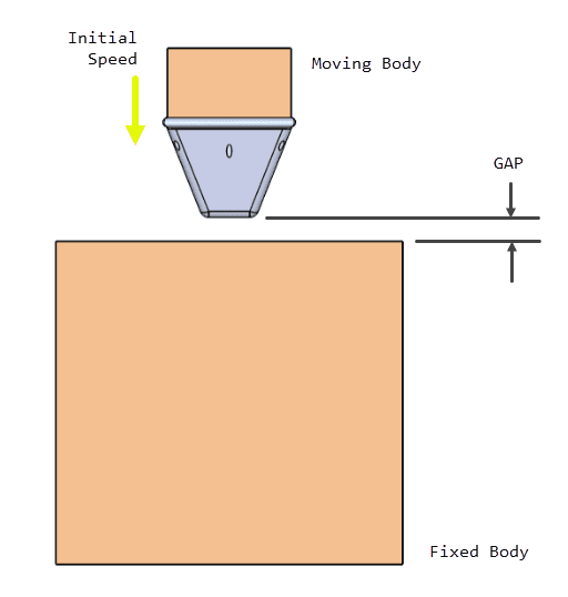
The two bodies are brought together by giving an initial speed to the moving body in the direction of the fixed body. Here, the objective of the simulation is to compute the deformation of the bodies due to the kinetic energy being converted into deformation.
The final speed before the impact is given by the following equation, which is the case of a free-fall drop of a body:
$$ v_i = \sqrt{ 2 g h } $$
Where \( g \) is the acceleration due to gravity and \( h \) is the drop height.
In order to save on computation time, the whole fall is not simulated, but the bodies are placed just before the impact occurs (with a separation gap), and the speed \( v_i \) is applied as an initial condition to the moving body.
Simulation Time Steps
The integration time step for the impact analysis must be small enough to properly capture the movement, peak stress, and physical contact development. The suggested criterion says that at first time step(s), physical contact should not occur, with the moving body still in the travel phase.
This can be computed by using the initial speed of the moving body and the gap:
$$ \Delta t_1 = \frac{ gap }{ v_i } $$
Where \( \Delta t_1 \) is the initial time step to be input for the simulation.
In the example case (see Figure 1), the initial speed and gap are 7 \(m/s\) and 0.0675 \(m\) respectively, so the computed \( \Delta t_1 \) is 0.00964 \(s\). This is split into approximately two, so the chosen initial time step is 0.005 \(s\).
Next is to determine the time step for the actual impact process. A good rule of thumb is to divide the initial time step into two to five equal steps to properly capture the physical contact process, deformation, and maximum stresses:
$$ \Delta t_2 = \frac{ \Delta t_1 }{ 2 \sim 5 } $$
If you find out that you get convergence problems or that you don’t get enough result steps during the impact process, try lowering the time step.
In the example case, the time step is first lowered from 0.005 to 0.002 \(s\), then further reduced to 0.001 \(s\). This allows us to properly capture the complete impact process.
Workbench Setup
Now that we have our planned time steps for the impact simulation, we proceed to set it up in the Workbench. First, we go to the Simulation Control panel and input the Simulation interval:
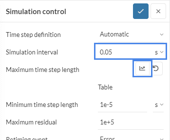
Then we press the Specify value button next to Maximum time step length to enter our time step scheme:
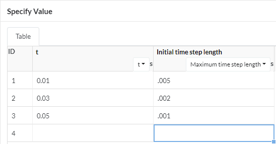
We use the table to specify the intervals and time steps. Here you can see we specified three consecutive intervals:
- Up to 0.01 \(s\), the time step is 0.005 \(s\),
- Up to 0.03 \(s\), the time step is 0.002 \(s\),
- Up to 0.05 \(s\), the time step is 0.001 \(s\).
You can input your computed time step scheme in a similar fashion!
Did you know?
The manual time step length assignment requires extra care. Please check this article to learn more about how to determine the manual time step length.
Important Information
If none of the above suggestions solved your problem, please post the issue in our forum or contact us.