Documentation
This validation case belongs to fluid dynamics. The aim of this test is to validate the following parameters for a compressible, steady-state turbulent flow through a de Laval Nozzle:
The simulation results from SimScale were compared to analytical results obtained from methods presented in [1].
A typical configuration of the de Laval nozzle with a non-smooth throat that was chosen as the geometry can be seen below:
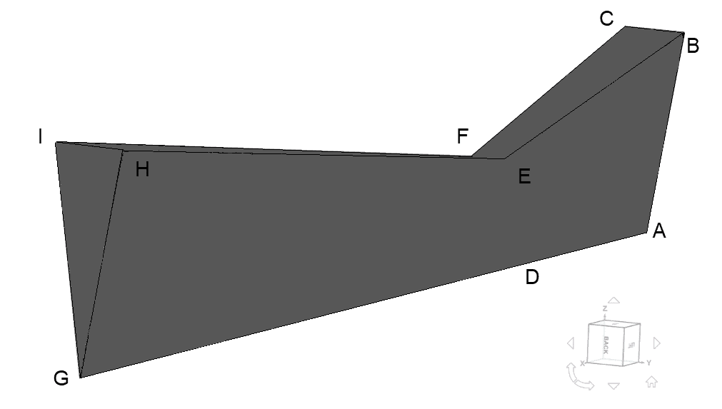
The nozzle is axisymmetric and an angular slice of the complete geometry with a wedge angle of 18\(°\) was used. The following table contains the coordinates of the reference points:
| Point | \(x\) \([mm]\) | \(y\) \([mm]\) | \(z\) \([mm]\) |
|---|---|---|---|
| A | 0 | 0 | 0 |
| B | 0 | 5.5434 | 35 |
| C | 0 | -5.5434 | 35 |
| D | 68.68 | 0 | 0 |
| E | 68.68 | 3.1677 | 20 |
| F | 68.68 | -3.1677 | 20 |
| G | 238.8 | 6.3354 | 40 |
| H | 238.8 | 0 | 0 |
| I | 238.8 | -6.3354 | 40 |
Tool Type: OpenFOAM®
Analysis type: Compressible with the k-omega SST turbulence model
Time dependency: Steady state
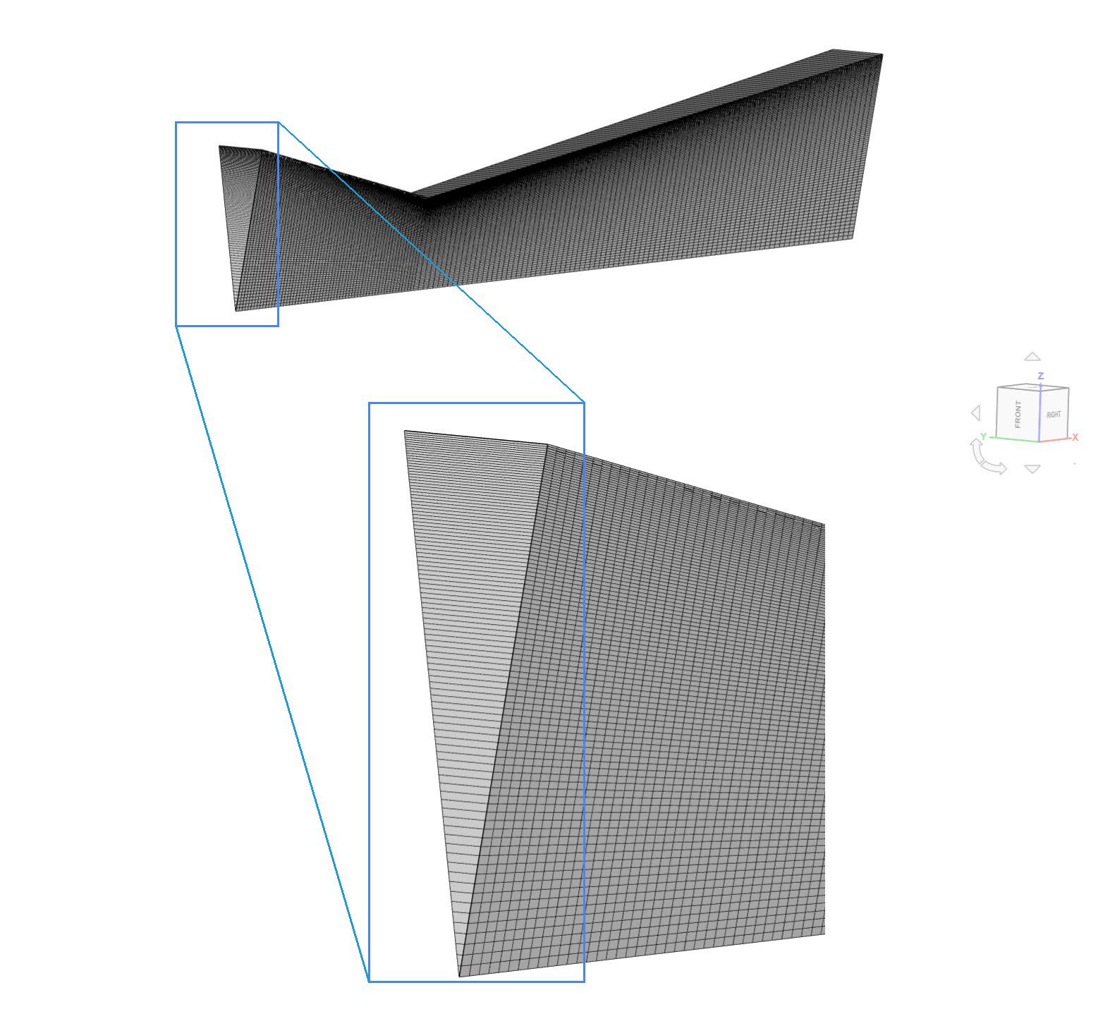
Mesh and Element types:
The hexahedral mesh was created externally and imported on to the SimScale platform, with an inflation of \(y^+\) = 30 near the walls, as the ‘wall functions’ model was chosen. To keep the flow two-dimensional, the mesh was designed to have only one layer in the \(y\) direction.
| Mesh type | Cells in the x-direction | Cells in the y-direction | Cells in the z–direction | Number of nodes | Type |
| blockMesh | 150 | 1 | 100 | 15000 | 2D Hex |
Fluid:
Boundary Conditions:
| Parameter | Inlet (ABC) | Outlet (GHI) | Wall (BEHIFC) | Wedges (AGHEB + AGIFC) |
| Velocity \([m/s]\) | 7.58 | Zero Gradient | No-slip | Wedge |
| Pressure \([Pa]\) | Zero Gradient | 1.3×10⁵ | Zero Gradient | Wedge |
| Temperature \([K]\) | 300 | Zero Gradient | Zero Gradient | Wedge |
| Turbulent kinetic energy \(k\) \([m^2/s^2]\) | 0.862 | Zero Gradient | Wall Function | Wedge |
| Specific dissipation rate \(ω\) \([s^{-1}]\) | 484.269 | Zero Gradient | Wall Function | Wedge |
| Turbulent thermal diffusivity \(α_t\) | Calculated | Calculated | Wall Function | Wedge |
| Turbulent dynamic viscosity \(μ_t\) | Calculated | Calculated | Wall Function | Wedge |
The wedge boundary condition is used in computational fluid dynamics to define an axisymmetric condition.
The results are calculated from Bernoulli’s equation and the ideal gas equation. The speed of sound can be calculated as:
$$c = \sqrt{\frac{\gamma RT}{m}} \tag{1}$$
Where:
The Mach number of a cutting plane be calculated as:
$$M = \frac{ U}{c} \tag{2}$$
Where:
Finally, the static pressure can be computed as:
$$P_{stat} = P_{stag}\ – \frac{1}{2}\rho \times U^2 \ \tag{3}$$
Where:
A comparison of the Mach number and pressure variation in the nozzle obtained with SimScale over the AG line with analytical results is given below:
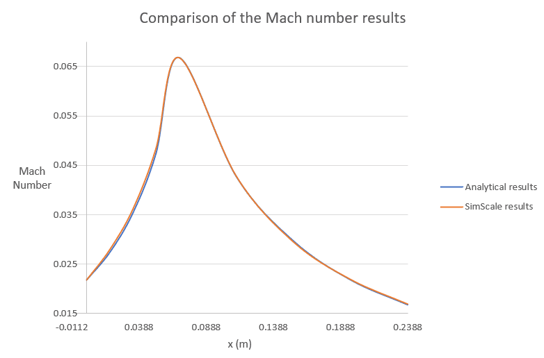
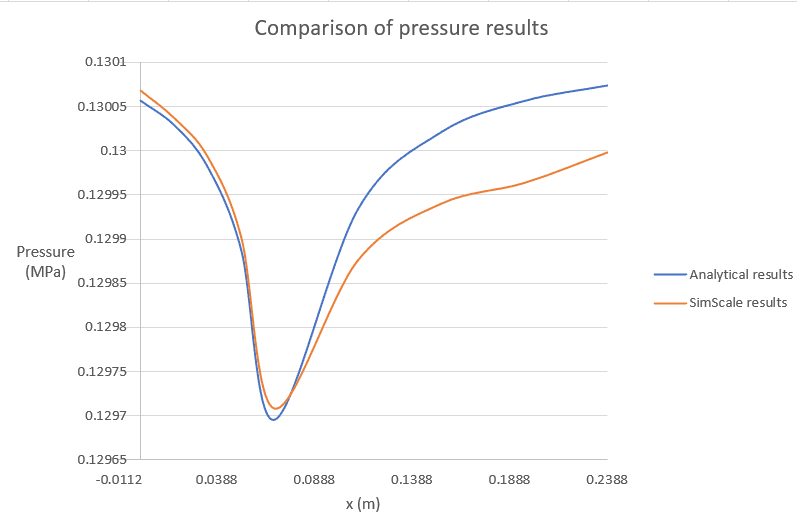
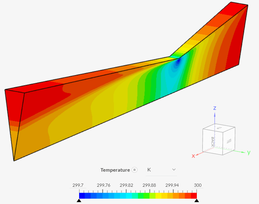
A source of deviation between the calculated and analytical results exists because the latter is calculated with a one-dimensional hypothesis. This means that all parameters are assumed to be uniform in the radial direction, while in the following figures, it seems that there exists radial variation too in the flow variables.
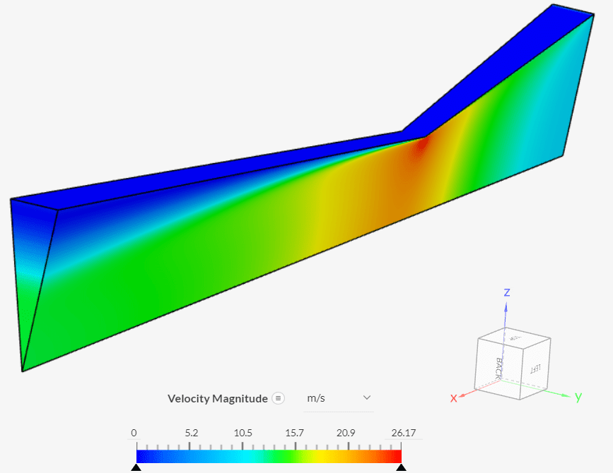
One can observe the radial variation causing results to slightly deviate:
Last updated: January 31st, 2023
We appreciate and value your feedback.
Sign up for SimScale
and start simulating now